Preregistration — fixed before any data was loaded61 lines
# Frozen before any data is loaded. Every cell below reads from PREREG,
# so no value is typed twice and the plan cannot drift from the code.
#
# Provenance of every parameter.
#
# From McConnell & Xu (2008), "Equity returns at the turn of the month",
# Financial Analysts Journal 64(2), 49-64, read out of the JSTOR copy on
# the author's Purdue page:
#   - day -1 is the last trading day of the prior month; days +1, +2 and +3
#     are the first three trading days of the month; the turn-of-the-month
#     interval is (-1, +3), four trading days
#   - "other days" is trading day -10 through -2 before month end and
#     trading day +4 through +10 after month start, which is the comparison
#     group and is deliberately not "every other day in the month"
#   - their sample is January 1926 to December 2005, which is where the
#     holdout starts
#   - the same window is attributed there to Lakonishok and Smidt (1988),
#     who ran it on the DJIA over 1897-1986. That paper is paywalled at
#     Oxford and was not fetched, so the window here is McConnell and Xu's
#     statement of it, not Lakonishok and Smidt's own text.
#
# Mine, not theirs, and named as mine:
#   - cost_bps, hac_lags, and the strategy test in "success". McConnell and
#     Xu measure the effect. They do not propose trading it.

PREREG = {
    "hypothesis": (
        "The mean daily US market return over the four-day turn-of-the-month "
        "interval exceeds the mean over McConnell and Xu's other-days window; "
        "the gap is still positive in the twenty years after their sample "
        "ends; and holding the market only on those four days beats "
        "buy-and-hold on Sharpe ratio in that holdout, net of costs."
    ),
    "universe": (
        "Ken French's daily US market factor, Mkt-RF plus RF, the total "
        "return on all CRSP NYSE, AMEX and NASDAQ common stocks. McConnell "
        "and Xu use CRSP value-weighted and equal-weighted indices directly; "
        "French's market factor is CRSP-based but separately constructed, so "
        "this is a close replication and not an exact one."
    ),
    "start":     "1926-07-01",
    "end":       "2026-06-30",
    "holdout":   "2006-01-01 onwards, touched once in the last cell of Results",
    "rebalance": "twice a month, into the market on day -1 and out after day +3",
    "params": {
        "tom_days":      [-1, 1, 2, 3],
        "other_days":    [-10, -9, -8, -7, -6, -5, -4, -3, -2, 4, 5, 6, 7, 8, 9, 10],
        "hac_lags":      5,
        "cost_bps":      10,
        "min_days_in_month": 15,
    },
    "success": (
        "All three must hold. (a) Over 1926-07 to 2005-12 the mean daily "
        "turn-of-the-month return exceeds the mean over other days, with "
        "|t| > 2 under Newey-West standard errors. (b) In the holdout the "
        "difference is still positive. (c) In the holdout, a strategy long "
        "the market on turn-of-the-month days and in Treasury bills "
        "otherwise has a higher Sharpe ratio than buy-and-hold, net of 10bp "
        "round-trip costs on 24 round trips a year."
    ),
}
Setup and imports21 lines
import sys
import warnings

# Library import notices are not findings, and they would otherwise be
# published as output. Silenced before the imports that raise them.
warnings.filterwarnings("ignore")

import numpy as np
import pandas as pd
import statsmodels.api as sm
import matplotlib.pyplot as plt

sys.path.append("..")
from lib import style, data

style.use()
SEED = 0
np.random.seed(SEED)

AS_OF = "2026-08-28"          # as-of date of every cached pull in this note
P = PREREG["params"]
Hypothesis
The US market earns most of its return on four trading days a month: the last day of one month and the first three of the next. That pattern is still there in the twenty years since the paper that measured it, and a strategy holding the market only on those days beats buying and holding.
McConnell and Xu (2008) found that over 1926 to 2005 investors "received no reward for bearing market risk except at turns of the month". This note tests their measurement on Ken French's daily market series, then asks what happened after their sample ended.
The test was fixed before any data was loaded. It is in the first cell, including the exact definition of both day windows, which are theirs, and the three conditions that all had to hold.
Prior work
McConnell, J. J. and Xu, W. (2008). Equity returns at the turn of the month. Financial Analysts Journal 64(2), 49-64. The paper this note tests. Every window definition here is theirs, read out of the article: day -1 is the last trading day of the prior month, days +1, +2 and +3 are the first three trading days of the month, and "other days" means trading day -10 through -2 before month end and +4 through +10 after month start. Their sample is January 1926 to December 2005, which is where the holdout begins.
Lakonishok, J. and Smidt, S. (1988). Are seasonal anomalies real? A ninety-year perspective. Review of Financial Studies 1(4), 403-425. The first report of the pattern, on the Dow Jones Industrial Average over 1897-1986. The paper is paywalled at Oxford and was not fetched, so the window used here is McConnell and Xu's statement of their definition rather than Lakonishok and Smidt's own text.
McLean, R. D. and Pontiff, J. (2016). Does academic research destroy stock return predictability? Journal of Finance 71(1), 5-32. Relevant to reading the holdout, and the reason it starts where the paper's sample ends.
Data
Ken French's data library, cached on 2026-08-28 under
research/data/famafrench/. One series: the daily research factors, 26,274
trading days from 1926-07-01 to 2026-06-30. The market total return is the
market excess return plus the risk-free rate, which is the return on all CRSP
NYSE, AMEX and NASDAQ common stocks. Returns are in percent.
Built from CRSP, so no survivorship bias enters through universe selection.
Two things to hold against the test.
The series is not the one they used. McConnell and Xu use the CRSP value-weighted and equal-weighted indices directly. French's market factor is CRSP-based but separately constructed. This is a close replication, not an exact one.
"Other days" is their window, not every other day. It covers trading days -10 to -2 and +4 to +10, so days in the middle of long months fall outside both groups and are excluded from the comparison. Roughly 2,400 of the 26,274 days are unclassified for that reason, plus any month with fewer than 15 trading days. Using their definition rather than a looser one is deliberate, since a comparison group that included the middle of the month would be a different test with a different answer.
Code24 lines
ffd = data.to_daily(data.famafrench("F-F_Research_Data_Factors_daily", AS_OF))
ffd = ffd.loc[PREREG["start"]:PREREG["end"]]
mkt = ffd["Mkt-RF"] + ffd["RF"]                      # total return, percent

# Trading-day position within the calendar month, counted from both ends.
grp   = mkt.groupby([mkt.index.year, mkt.index.month])
from_start = grp.cumcount() + 1                      # +1 is the first trading day
month_len  = grp.transform("size")
from_end   = from_start - month_len - 1              # -1 is the last trading day

fwd = from_start.where(from_start <= 10)
bwd = from_end.where(from_end >= -10)
long_enough = month_len >= P["min_days_in_month"]

is_tom   = (fwd.isin([d for d in P["tom_days"] if d > 0]) |
            bwd.isin([d for d in P["tom_days"] if d < 0])) & long_enough
is_other = ((fwd.isin([d for d in P["other_days"] if d > 0]) |
             bwd.isin([d for d in P["other_days"] if d < 0])) & long_enough & ~is_tom)

print(f"daily factors   {len(ffd):6,} rows  {ffd.index.min().date()} -> {ffd.index.max().date()}")
print(f"turn-of-month days {int(is_tom.sum()):6,}")
print(f"other days         {int(is_other.sum()):6,}")
print(f"unclassified       {int((~(is_tom | is_other)).sum()):6,}")
print(f"missing values: {int(ffd.isna().sum().sum())}")
daily factors 26,274 rows 1926-07-01 -> 2026-06-30 turn-of-month days 4,800 other days 19,061 unclassified 2,413 missing values: 0
Method
Every trading day is labelled by its position in the calendar month, counted forward from the first trading day and backward from the last. Day -1 is the last trading day of a month, so the four-day turn runs -1, +1, +2, +3 and straddles the month boundary.
The test regresses the daily market return on a constant and a turn-of-the-month dummy, over the days belonging to either window. The dummy's coefficient is the difference in mean daily return. Standard errors are Newey-West at five lags, which covers one trading week.
Three preregistered conditions, all of which had to hold:
- (a) the difference is positive with |t| above 2 over 1926-07 to 2005-12
- (b) the difference is still positive in the holdout
- (c) in the holdout, holding the market only on turn-of-the-month days and Treasury bills otherwise beats buy-and-hold on Sharpe ratio, net of 10bp round trips, of which there are 24 a year
Code27 lines
def tom_gap(sl, lags=P["hac_lags"]):
    """Mean daily return on turn-of-month days minus other days."""
    m, t_, o_ = mkt.loc[sl], is_tom.loc[sl], is_other.loc[sl]
    use = t_ | o_
    y = m[use]
    X = sm.add_constant(pd.DataFrame({"tom": t_[use].astype(float)}, index=y.index))
    fit = sm.OLS(y, X).fit(cov_type="HAC", cov_kwds={"maxlags": lags})
    return {"tom": m[t_].mean(), "other": m[o_].mean(),
            "gap": fit.params["tom"], "t": fit.tvalues["tom"],
            "n_tom": int(t_.sum()), "n_other": int(o_.sum())}

def strategy(sl, cost_bps=P["cost_bps"]):
    """Long the market on turn-of-month days, Treasury bills otherwise."""
    m  = mkt.loc[sl] / 100.0
    rf = ffd["RF"].loc[sl] / 100.0
    w  = is_tom.loc[sl].astype(float)
    net = w * m + (1 - w) * rf - w.diff().abs().fillna(0) * cost_bps / 10000.0
    return net, m, rf

def sharpe(x, rf):
    return np.sqrt(252) * (x - rf).mean() / (x - rf).std()

def annualised(x):
    return ((1 + x).prod() ** (252 / len(x)) - 1) * 100

IN  = slice(None, "2005-12-31")
OUT = slice("2006-01-01", None)
Results
Code11 lines
# Criterion (a): is the turn-of-month premium there in sample?

print("mean daily market return, percent\n")
print(f"{'period':32} {'TOM n':>7} {'TOM':>9} {'other':>9} {'gap':>9} {'t':>7}")
for label, sl in [("in sample  1926-07 to 2005-12", IN),
                  ("full sample 1926-07 to 2026-06", slice(None))]:
    d = tom_gap(sl)
    print(f"{label:32} {d['n_tom']:>7,} {d['tom']:+9.4f} {d['other']:+9.4f} "
          f"{d['gap']:+9.4f} {d['t']:+7.2f}")

d_in = tom_gap(IN)
mean daily market return, percent period TOM n TOM other gap t in sample 1926-07 to 2005-12 3,816 +0.1614 +0.0128 +0.1487 +8.03 full sample 1926-07 to 2026-06 4,800 +0.1391 +0.0189 +0.1202 +7.12
Criterion (a) passes by a wide margin. Over the eighty years to 2005, the four turn-of-the-month days averaged +0.161% and the other days +0.013%, a gap of +0.149% a day at t = 8.03.
The second number is the one that makes this anomaly unusual. On the other sixteen days of McConnell and Xu's window the market returned about a hundredth of a percent a day, which is close to the risk-free rate and not close to an equity premium. Their sentence about investors receiving no reward for market risk except at turns of the month is not rhetoric. It is what the column says.
Code17 lines
fig, ax = plt.subplots(figsize=(8, 4.3))

days = [d for d in range(-10, 0)] + [d for d in range(1, 11)]
means, labels = [], []
for d in days:
    sel = (bwd == d) if d < 0 else (fwd == d)
    sel = sel & long_enough
    means.append(mkt[sel].mean())
    labels.append(f"{d:+d}")

colors = [style.ACCENT if d in P["tom_days"] else style.SERIES[2] for d in days]
ax.bar(labels, means, color=colors, width=0.7)
ax.axhline(0, color=style.MUTED, lw=0.7)
ax.set_xlabel("Trading day of the month. Negative counts back from the last day.")
ax.set_ylabel("Mean daily return, %")
ax.set_title("The four turn-of-the-month days, 1926-2026, in accent")
plt.show()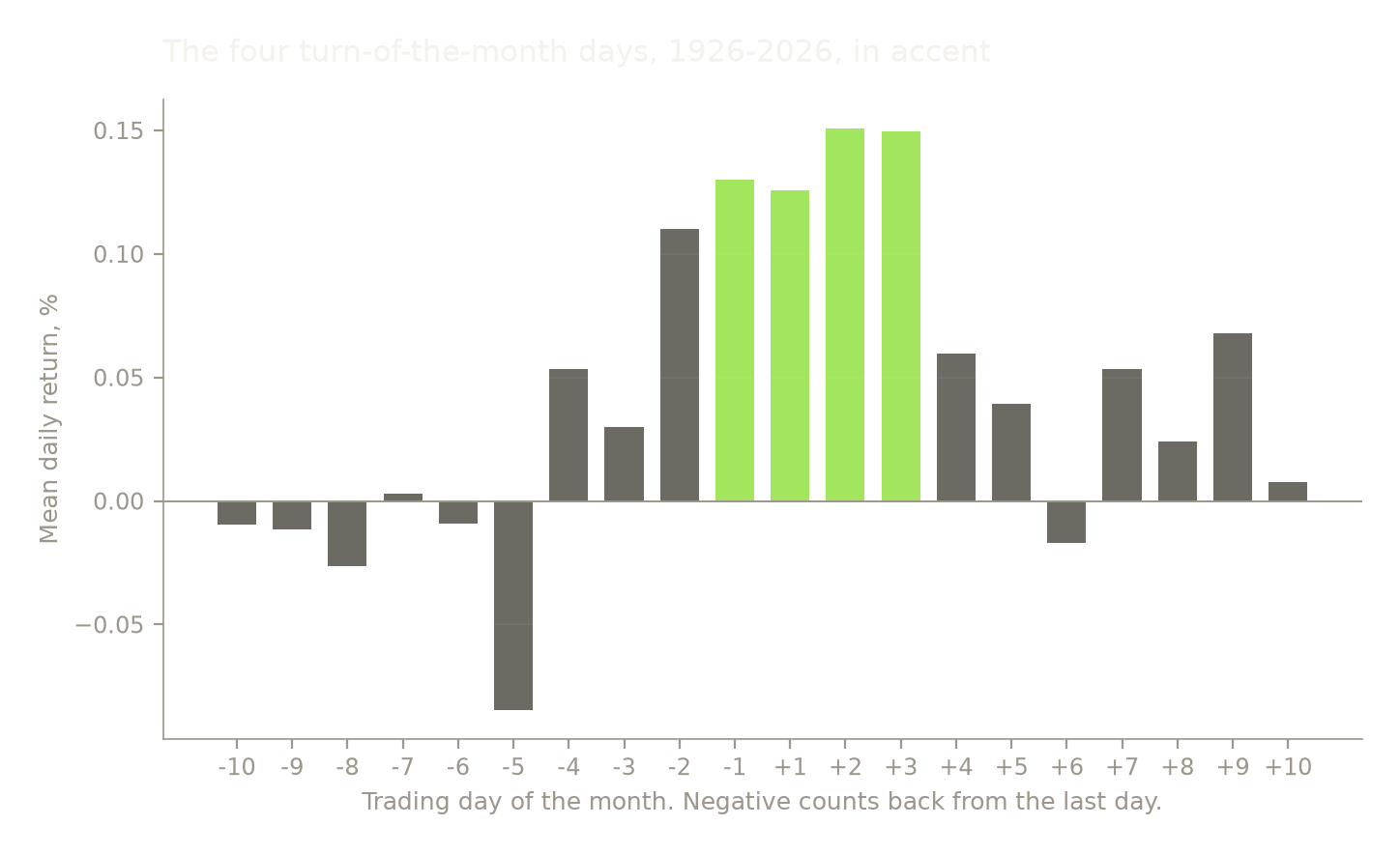
The four accent bars sit at the top of a hump rather than inside a fence. Day -2 averages +0.110%, close behind day -1, so the run-up starts a day before the window opens. On the other side the decay is uneven: day +9 averages +0.068%, more than day +4.
The bars on the left are the more surprising part. Days -10 through -5 average at or below zero, and day -5 is the worst day of the month at -0.085%. The week before the turn does not merely earn less than the turn. It loses money.
Code18 lines
# Criteria (b) and (c): the holdout. Evaluated once.

d_out = tom_gap(OUT)
net_out, mkt_out, rf_out = strategy(OUT)

print(f"holdout 2006-01 to 2026-06\n")
print(f"  turn-of-month days   {d_out['tom']:+.4f}%   n {d_out['n_tom']:,}")
print(f"  other days           {d_out['other']:+.4f}%   n {d_out['n_other']:,}")
print(f"  gap                  {d_out['gap']:+.4f}%   t {d_out['t']:+.2f}")
print()
print(f"  strategy      annualised {annualised(net_out):+6.2f}%   "
      f"Sharpe {sharpe(net_out, rf_out):+.3f}")
print(f"  buy and hold  annualised {annualised(mkt_out):+6.2f}%   "
      f"Sharpe {sharpe(mkt_out, rf_out):+.3f}")
print()
print(f"  in sample gap {d_in['gap']:+.4f}% (t {d_in['t']:+.2f})   "
      f"holdout gap {d_out['gap']:+.4f}% (t {d_out['t']:+.2f})")
print(f"  the holdout retains {100 * d_out['gap'] / d_in['gap']:.0f}% of the in-sample gap")
holdout 2006-01 to 2026-06 turn-of-month days +0.0523% n 984 other days +0.0425% n 3,905 gap +0.0098% t +0.24 strategy annualised +1.16% Sharpe -0.026 buy and hold annualised +11.39% Sharpe +0.561 in sample gap +0.1487% (t +8.03) holdout gap +0.0098% (t +0.24) the holdout retains 7% of the in-sample gap
Criterion (b) passes on a technicality and criterion (c) fails outright.
The holdout gap is +0.0098% a day at t = 0.24. It is positive, which is what the criterion asked, and it is 7% of the in-sample gap. Turn-of-the-month days returned +0.052% and other days +0.043%, which is as close to no difference as this kind of test produces.
The strategy is worse than that. Holding the market only on turn days returned 1.16% a year against 11.39% for buying and holding, with a Sharpe ratio of -0.03 against +0.56.
An anomaly that survived at t above 4 in each of three consecutive quarter-centuries is, on this evidence, no longer there.
Code20 lines
fig, ax = plt.subplots(figsize=(8, 4.3))

for sl, label, colour, width in [
    (IN,  "1926-07 to 2005-12", style.ACCENT,     1.8),
    (OUT, "2006-01 to 2026-06", style.SERIES[1],  1.2),
]:
    ys = []
    for d in days:
        sel = ((bwd == d) if d < 0 else (fwd == d)) & long_enough
        ys.append(mkt.loc[sl][sel.loc[sl]].mean())
    ax.plot(labels, ys, color=colour, lw=width, marker="o", ms=3.5, label=label)

ax.axhline(0, color=style.MUTED, lw=0.7)
for d in P["tom_days"]:
    ax.axvline(labels[days.index(d)], color=style.SUBTLE, alpha=0.16, lw=9)
ax.set_xlabel("Trading day of the month. Negative counts back from the last day.")
ax.set_ylabel("Mean daily return, %")
ax.set_title("The turn-of-the-month hump, before and after 2006")
ax.legend(loc="upper right")
plt.show()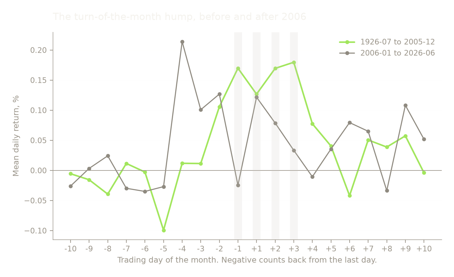
The shaded columns are the four turn days. The accent line sits high and level across all four, between +0.127% and +0.180%.
The grey line has no hump there. It is negative on day -1, the single best day of the old profile, and its highest point is day -4 at +0.214%, four days before the window opens. Some of that is noise: twenty years gives 246 observations per bucket against 954 for the eighty before it, so each grey point carries about twice the standard error of an accent one. What is not noise is the absence of any elevation across the four shaded columns.
Code16 lines
fig, ax = plt.subplots(figsize=(8, 4.3))

net_all, mkt_all, rf_all = strategy(slice(None))
ax.plot(net_all.index, (1 + net_all).cumprod(), color=style.ACCENT, lw=1.6,
        label="In the market on turn-of-month days only")
ax.plot(mkt_all.index, (1 + mkt_all).cumprod(), color=style.SERIES[1], lw=1.2,
        label="Buy and hold")
ax.axvspan(pd.Timestamp("2006-01-01"), net_all.index.max(),
           color=style.SUBTLE, alpha=0.14, lw=0)
ax.annotate("holdout", (pd.Timestamp("2007-06-30"), 3),
            fontsize=8.5, color=style.MUTED)
ax.set_yscale("log")
ax.set_ylabel("Growth of $1, log scale")
ax.set_title("Trading the turn of the month, net of 10bp round trips")
ax.legend(loc="upper left")
plt.show()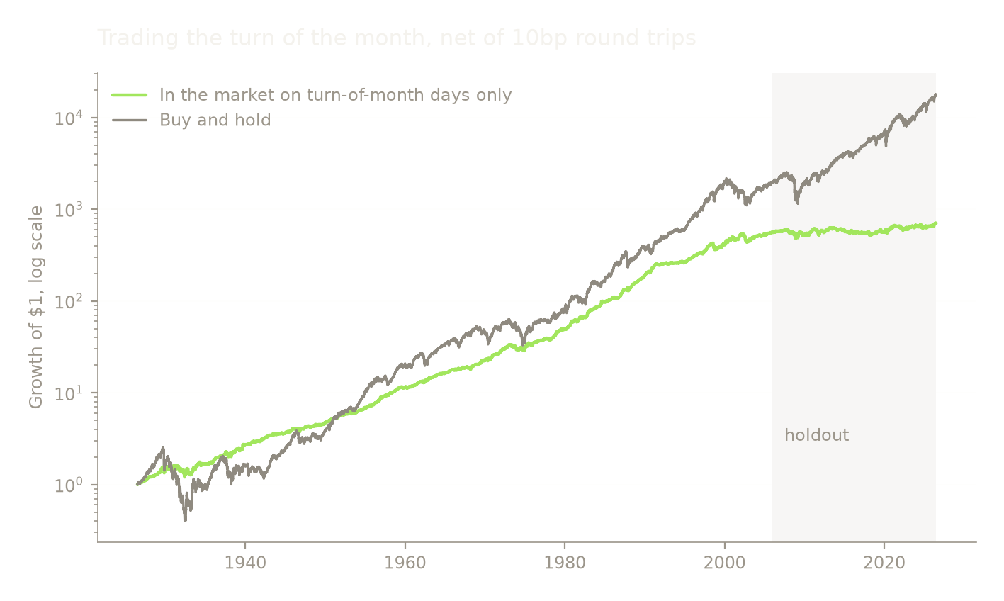
The accent line is invested 18% of the time and rises almost as smoothly as a bond ladder, sitting out the 1930s and 1974 drawdowns that the grey line takes in full. That is the appeal of the anomaly, and it is why its in-sample Sharpe ratio of 0.66 beats the market's 0.43 despite ending lower.
Then it stops. A dollar reaches 557 by the end of 2005 and 705 today, while buy-and-hold goes from 1,946 to 17,678 over the same twenty years.
What broke
Code9 lines
# Subperiod behaviour, by 25-year block.

print(f"{'period':14} {'TOM%':>9} {'other%':>9} {'gap%':>9} {'t':>7}")
for y0 in [1926, 1951, 1976, 2001]:
    sl = slice(f"{y0}-01-01", f"{y0 + 24}-12-31")
    if len(mkt.loc[sl]) > 500:
        d = tom_gap(sl)
        print(f"{y0}-{y0 + 24}  {d['tom']:+9.4f} {d['other']:+9.4f} "
              f"{d['gap']:+9.4f} {d['t']:+7.2f}")
period TOM% other% gap% t 1926-1950 +0.1851 +0.0050 +0.1801 +4.48 1951-1975 +0.1487 +0.0108 +0.1379 +5.32 1976-2000 +0.1681 +0.0276 +0.1404 +4.62 2001-2025 +0.0525 +0.0322 +0.0204 +0.55
Code16 lines
fig, ax = plt.subplots(figsize=(8, 3.9))

blocks, gaps, sig = [], [], []
for y0 in [1926, 1951, 1976, 2001]:
    sl = slice(f"{y0}-01-01", f"{y0 + 24}-12-31")
    d = tom_gap(sl)
    blocks.append(f"{y0}-{y0 + 24}")
    gaps.append(d["gap"])
    sig.append(abs(d["t"]) > 2)

ax.bar(blocks, gaps, color=[style.ACCENT if s else style.SERIES[2] for s in sig],
       width=0.55)
ax.axhline(0, color=style.MUTED, lw=0.7)
ax.set_ylabel("Turn-of-month minus other days, % per day")
ax.set_title("Blocks reaching |t| > 2 on their own, in accent")
plt.show()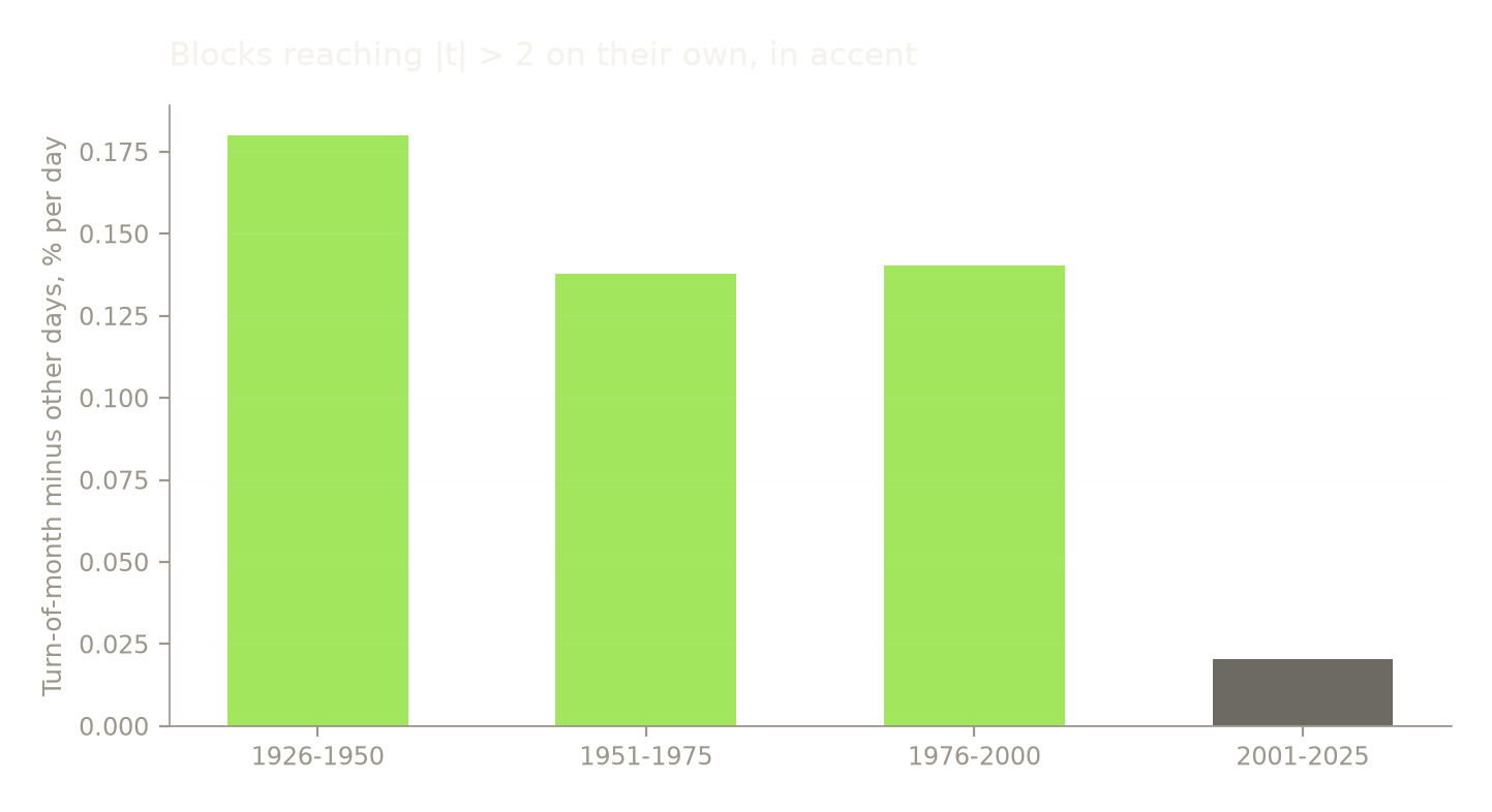
Three consecutive quarter-centuries at +0.18%, +0.14% and +0.14% a day, each clearing t = 4 on its own, and then +0.02% at t = 0.55. This is not a premium that faded. It stopped.
The break lands close to 2001, which is when US exchanges finished converting to decimal pricing and the minimum quote increment fell from a sixteenth of a dollar to a penny. That timing is suggestive and this note does not test it. Nothing here separates decimalisation from index-fund flows, from electronic market making, or from the effect having been published often enough to be traded away.
Code7 lines
# Cost sensitivity in the holdout. The strategy trades 24 times a year.

print(f"holdout, buy-and-hold Sharpe {sharpe(mkt_out, rf_out):+.3f}\n")
for c in [0, 10, 25, 50]:
    n, _, rfc = strategy(OUT, cost_bps=c)
    print(f"  {c:3d}bp round trip   annualised {annualised(n):+6.2f}%   "
          f"Sharpe {sharpe(n, rfc):+.3f}")
holdout, buy-and-hold Sharpe +0.561
0bp round trip annualised +3.62% Sharpe +0.265
10bp round trip annualised +1.16% Sharpe -0.026
25bp round trip annualised -2.43% Sharpe -0.458
50bp round trip annualised -8.15% Sharpe -1.143
Costs are not what kills it in the holdout, though they finish it off. At zero cost the strategy still returns 3.62% a year with a Sharpe ratio of 0.27, against 0.56 for buying and holding. The 10bp round trip takes another 2.5 percentage points a year, because 24 round trips a year at 10bp is 2.4% of capital before any slippage.
That last figure is the practical objection to the anomaly even in the period when it worked. A premium of 0.149% a day over four days is about 0.6% a month gross, and the trading needed to capture it costs a meaningful share of that.
Verdict
Do not trade it. One of three preregistered conditions fails and the second passes only on its sign.
The in-sample result is as strong as replications get. Over eighty years the four turn-of-the-month days returned +0.161% a day against +0.013% on the comparison days, a gap of +0.149% at t = 8.03, and the pattern clears t = 4 in each of three consecutive quarter-centuries. McConnell and Xu's claim that investors were paid for market risk only at turns of the month replicates on French's series without qualification.
Since 2006 it is gone. The gap is +0.0098% a day at t = 0.24, which is 7% of what it was, and the day-by-day profile is flat where it used to have a hump. The strategy returned 1.16% a year against 11.39% for holding the market.
The break is close enough to 2001 to invite the decimalisation explanation, and this note gives no evidence for it. What the note does establish is narrower and more useful: one of the most statistically robust calendar anomalies ever documented has produced nothing for twenty years, and a reader deciding whether to act on the published evidence should know that the published evidence stops in 2005.
References
French, K. R. (2026). Fama/French 3 factors, daily. Data library, accessed 2026-08-28. https://mba.tuck.dartmouth.edu/pages/faculty/ken.french/data_library.html
Lakonishok, J. and Smidt, S. (1988). Are seasonal anomalies real? A ninety-year perspective. The Review of Financial Studies 1(4), 403-425. https://academic.oup.com/rfs/article-abstract/1/4/403/1566965
McConnell, J. J. and Xu, W. (2008). Equity returns at the turn of the month. Financial Analysts Journal 64(2), 49-64. https://rpc.cfainstitute.org/research/financial-analysts-journal/2008/equity-returns-at-the-turn-of-the-month The copy read for this note, and the source of every window definition above: https://business.purdue.edu/faculty/mcconnell/publications/Equity-Returns-at-the-Turn-of-the-Month.pdf
McLean, R. D. and Pontiff, J. (2016). Does academic research destroy stock return predictability? Journal of Finance 71(1), 5-32. https://onlinelibrary.wiley.com/doi/10.1111/jofi.12365
Code6 lines
print(f"python       {sys.version.split()[0]}")
print(f"pandas       {pd.__version__}")
print(f"numpy        {np.__version__}")
print(f"statsmodels  {sm.__version__}")
print(f"seed         {SEED}")
print(f"data as-of   {AS_OF}  (research/data/famafrench/{AS_OF}/)")
python 3.12.13 pandas 3.0.5 numpy 2.5.2 statsmodels 0.15.0 seed 0 data as-of 2026-08-28 (research/data/famafrench/2026-08-28/)