Preregistration — fixed before any data was loaded66 lines
# Frozen before any data is loaded. Every cell below reads from PREREG,
# so no value is typed twice and the plan cannot drift from the code.
#
# Provenance of every parameter.
#
# From Jegadeesh (1990), "Evidence of predictable behavior of security
# returns", Journal of Finance 45(3), 881-898, read from the Wiley abstract
# page. The full text was not fetched: two hosts returned 403 and 425.
# What the abstract page supports:
#   - the effect: significant negative first-order serial correlation in
#     monthly stock returns
#   - ten portfolios formed on one-month-ahead forecasts, extreme decile
#     spread of 2.49% a month over 1934-1987
#
# Nothing else here is his. In particular:
#   - French's ST_Rev factor is not Jegadeesh's portfolio. It is a
#     value-weighted long-short on the 30th and 70th NYSE percentiles of the
#     prior month's return, crossed with the NYSE size median. Terciles, not
#     deciles. The note reports on French's factor and says so.
#   - the split date is mine. Journal of Finance 45(3) is a 1990 issue but
#     the issue month was not verified, so the cutoff is the end of the
#     publication year rather than an invented month.
#   - turnover_legs, the cost grid, hac_lags and "success" are mine.
#
# The strategy replaces both legs every month, so the honest question is not
# only whether the gross premium shrank but at what cost level it dies. Both
# are preregistered.

PREREG = {
    "hypothesis": (
        "Ken French's short-term reversal factor earned a positive average "
        "monthly return before Jegadeesh was published, its average in the "
        "period after publication is lower, and the round-trip cost at which "
        "the strategy breaks even in that later period is below 25 basis "
        "points, which would mean it is no longer investable."
    ),
    "universe": (
        "Ken French's F-F_ST_Reversal_Factor, a value-weighted long-short "
        "built from six portfolios: NYSE, AMEX and NASDAQ stocks split at "
        "the NYSE size median and at the 30th and 70th NYSE percentiles of "
        "the prior month's return. Rebuilt monthly. Built from CRSP, so no "
        "survivorship bias in universe selection. The factor is gross of "
        "trading costs, which is the whole reason for the cost grid below."
    ),
    "start":     "1926-02-28",
    "end":       "2026-06-30",
    "holdout":   "1991-01-31 onwards, touched once in the last cell of Results",
    "rebalance": "monthly, both legs replaced in full",
    "params": {
        "pre_pub_end":   "1990-12-31",   # end of Jegadeesh's publication year
        "turnover_legs": 2.0,            # long and short both replaced each month
        "cost_grid_bps": [0, 10, 25, 50, 100],
        "hac_lags":      6,
        "decade_panel":  True,
    },
    "success": (
        "All three must hold for the decay claim to stand. (a) Over "
        "1926-02 to 1990-12 the factor has a positive gross mean monthly "
        "return with |t| > 2 under Newey-West standard errors. (b) In the "
        "holdout the gross mean is lower than the pre-publication mean. "
        "(c) In the holdout the breakeven round-trip cost is under 25 basis "
        "points. A decade panel is reported either way, so the reader sees "
        "when the change happened rather than only that a two-way split "
        "differs."
    ),
}
Setup and imports21 lines
import sys
import warnings

# Library import notices are not findings, and they would otherwise be
# published as output. Silenced before the imports that raise them.
warnings.filterwarnings("ignore")

import numpy as np
import pandas as pd
import statsmodels.api as sm
import matplotlib.pyplot as plt

sys.path.append("..")
from lib import style, data

style.use()
SEED = 0
np.random.seed(SEED)

AS_OF = "2026-08-28"          # as-of date of every cached pull in this note
P = PREREG["params"]
Hypothesis
Stocks that fell last month tend to bounce next month. Acting on that means replacing the entire portfolio every month, so the premium has to clear an unusually high trading cost before any of it reaches the investor. Where that break-even sits today is what this note measures.
Jegadeesh (1990) documented monthly return reversal and reported a 2.49% spread between extreme decile portfolios over 1934-1987. This note asks a narrower and more practical question on Ken French's reversal factor: not whether the premium shrank, but at what round-trip cost it goes to zero, and whether that number is still above anything a real desk could trade at.
The test was fixed before any data was loaded, including the cost grid, the turnover assumption, and the 25 basis point threshold that decides the verdict.
Prior work
Jegadeesh, N. (1990). Evidence of predictable behavior of security returns. The Journal of Finance 45(3), 881-898. The origin of the effect. The full text could not be fetched: two hosts returned 403 and 425. The Wiley abstract page supports the citation, the significant negative first-order serial correlation in monthly returns, and the 2.49% monthly spread between extreme decile portfolios over 1934-1987. Nothing else in this note is attributed to him, and the portfolio tested here is not his.
Lehmann, B. N. (1990). Fads, martingales, and market efficiency. Quarterly Journal of Economics 105(1), 1-28. The other 1990 paper on short-horizon reversal, at weekly frequency. Not tested here, and named because a reader looking for the origin of this effect will meet both.
McLean, R. D. and Pontiff, J. (2016). Does academic research destroy stock return predictability? Journal of Finance 71(1), 5-32. Their average predictor loses 58% of its return after publication. Reversal is a useful case for that claim precisely because its costs are so high that publication is not the only candidate explanation.
Data
Ken French's data library, cached on 2026-08-28 under
research/data/famafrench/. The monthly short-term reversal factor, 1,205
months from 1926-02 to 2026-06, and the monthly research factors. Returns are
in percent.
French builds the factor from six value-weighted portfolios: NYSE, AMEX and NASDAQ stocks split at the NYSE size median and at the 30th and 70th NYSE percentiles of the prior month's return. It is long the low prior-return portfolios and short the high ones, rebuilt monthly. Built from CRSP, so no survivorship bias enters through universe selection.
Three limits on what this can show.
It is not Jegadeesh's portfolio. He forms ten portfolios from a return forecast. French sorts into terciles on last month's return alone. Terciles are far less extreme than deciles, so the premium here should be smaller than his 2.49% by construction, and the two numbers are never compared below.
The factor is gross. French charges nothing for trading, and this strategy replaces both legs every month. That is the reason the whole note is organised around a cost grid rather than a single net number.
The turnover assumption is mine. Two legs fully replaced each month is treated as 2.0 round trips of turnover. It is a simplification: some names persist in the same tercile from one month to the next, so the true figure is lower, and every breakeven cost below is therefore conservative in the strategy's favour.
Code14 lines
st = data.to_month_end(data.famafrench("F-F_ST_Reversal_Factor", AS_OF))
ff = data.to_month_end(data.famafrench("F-F_Research_Data_Factors", AS_OF))

st = st.loc[PREREG["start"]:PREREG["end"]]
ff = ff.loc[PREREG["start"]:PREREG["end"]]
rev = st["ST_Rev"]

PRE = slice(None, P["pre_pub_end"])
OUT = slice("1991-01-01", None)

print(f"reversal factor  {len(rev):6,} rows  {rev.index.min().date()} -> {rev.index.max().date()}")
print(f"research factors {len(ff):6,} rows  {ff.index.min().date()} -> {ff.index.max().date()}")
print(f"pre-publication {len(rev.loc[PRE]):,} months     holdout {len(rev.loc[OUT]):,} months")
print(f"missing values: {int(rev.isna().sum())}")
reversal factor 1,205 rows 1926-02-28 -> 2026-06-30 research factors 1,200 rows 1926-07-31 -> 2026-06-30 pre-publication 779 months holdout 426 months missing values: 0
Method
The factor return is gross, so a net return is the gross return minus turnover times the round-trip cost:
net = gross - 2.0 * cost_bps / 100
with the 2.0 coming from replacing both legs each month and the division by 100 converting basis points to the percent units French uses.
Turning that around gives the number the note is built on. The breakeven round-trip cost is the cost at which the net mean return is exactly zero:
breakeven_bps = 100 * mean_gross / 2.0
That single figure says what a gross Sharpe ratio cannot: whether a desk paying realistic costs would have made anything. Means are tested against zero with Newey-West standard errors at six lags.
Three preregistered conditions, all of which had to hold:
- (a) the gross mean is positive with |t| above 2 over 1926-02 to 1990-12
- (b) the holdout gross mean is below the pre-publication mean
- (c) the holdout breakeven cost is under 25 basis points
Code11 lines
def mean_t(x, lags=P["hac_lags"]):
    """Mean and its Newey-West t-statistic against zero."""
    fit = sm.OLS(x.values, np.ones(len(x))).fit(cov_type="HAC", cov_kwds={"maxlags": lags})
    return len(x), x.mean(), float(fit.tvalues[0]), np.sqrt(12) * x.mean() / x.std()

def net_of(x, cost_bps):
    return x - P["turnover_legs"] * cost_bps / 100.0

def breakeven_bps(x):
    """Round-trip cost, in basis points, at which the mean net return is zero."""
    return 100.0 * x.mean() / P["turnover_legs"]
Results
Code11 lines
# Criterion (a): was the gross premium there before publication?

print("Ken French short-term reversal factor, gross of costs\n")
print(f"{'period':40} {'n':>5} {'mean%':>8} {'t':>7} {'Sharpe':>8}")
for label, sl in [("pre-publication  1926-02 to 1990-12", PRE),
                  ("full sample      1926-02 to 2026-06", slice(None))]:
    n, mu, t, sr = mean_t(rev.loc[sl])
    print(f"{label:40} {n:>5} {mu:+8.3f} {t:+7.2f} {sr:+8.3f}")

n_p, mu_p, t_p, sr_p = mean_t(rev.loc[PRE])
print(f"\nbreakeven round-trip cost, pre-publication: {breakeven_bps(rev.loc[PRE]):.1f} bps")
Ken French short-term reversal factor, gross of costs period n mean% t Sharpe pre-publication 1926-02 to 1990-12 779 +0.884 +6.34 +0.899 full sample 1926-02 to 2026-06 1205 +0.622 +5.79 +0.622 breakeven round-trip cost, pre-publication: 44.2 bps
Criterion (a) passes. Before publication the factor returned +0.88% a month gross at t = 6.34, with a gross Sharpe ratio of 0.90. On the gross numbers this is one of the strongest premiums in the factor literature.
The breakeven figure is the first sign of trouble, and it is in the period when the effect supposedly worked. At 44 basis points round trip the whole premium is gone. A strategy replacing its entire book every month at 44bp was not obviously tradeable in 1960, let alone attractive.
Code14 lines
# Criteria (b) and (c): the holdout. Evaluated once.

n_h, mu_h, t_h, sr_h = mean_t(rev.loc[OUT])
be_h = breakeven_bps(rev.loc[OUT])

print(f"holdout 1991-01 to 2026-06, n {n_h} months\n")
print(f"  gross mean     {mu_h:+.3f}% per month")
print(f"  t              {t_h:+.2f}")
print(f"  gross Sharpe   {sr_h:+.3f}")
print(f"  breakeven cost {be_h:.1f} bps round trip")
print()
print(f"  pre-publication: mean {mu_p:+.3f}%  t {t_p:+.2f}  breakeven {breakeven_bps(rev.loc[PRE]):.1f} bps")
print(f"  holdout:         mean {mu_h:+.3f}%  t {t_h:+.2f}  breakeven {be_h:.1f} bps")
print(f"  the holdout retains {100 * mu_h / mu_p:.0f}% of the pre-publication mean")
holdout 1991-01 to 2026-06, n 426 months gross mean +0.143% per month t +0.97 gross Sharpe +0.140 breakeven cost 7.1 bps round trip pre-publication: mean +0.884% t +6.34 breakeven 44.2 bps holdout: mean +0.143% t +0.97 breakeven 7.1 bps the holdout retains 16% of the pre-publication mean
Criteria (b) and (c) both pass. The holdout gross mean is +0.14% a month against +0.88% before publication, 16% of what it was and no longer distinguishable from zero at t = 0.97.
The breakeven cost is 7.1 basis points round trip. That is the number that settles it. A monthly-rebalanced long-short in the tails of the return distribution does not trade at 7bp all-in, in 1991 or now, so there has been nothing here to capture for thirty-five years.
All three preregistered conditions hold. The hypothesis is confirmed.
Code19 lines
fig, ax = plt.subplots(figsize=(8, 4.3))

for cost, colour, width, label in [
    (0,  style.ACCENT,    1.7, "Gross, no costs"),
    (10, style.SERIES[1], 1.2, "10bp round trip"),
    (25, style.SERIES[2], 1.2, "25bp round trip"),
]:
    g = (1 + net_of(rev, cost) / 100).cumprod()
    ax.plot(g.index, g.values, color=colour, lw=width, label=label)

ax.axvspan(pd.Timestamp("1991-01-31"), rev.index.max(),
           color=style.SUBTLE, alpha=0.14, lw=0)
ax.annotate("holdout", (pd.Timestamp("1993-06-30"), 0.6),
            fontsize=8.5, color=style.MUTED)
ax.set_yscale("log")
ax.set_ylabel("Growth of $1, log scale")
ax.set_title("Short-term reversal at three cost assumptions")
ax.legend(loc="upper left")
plt.show()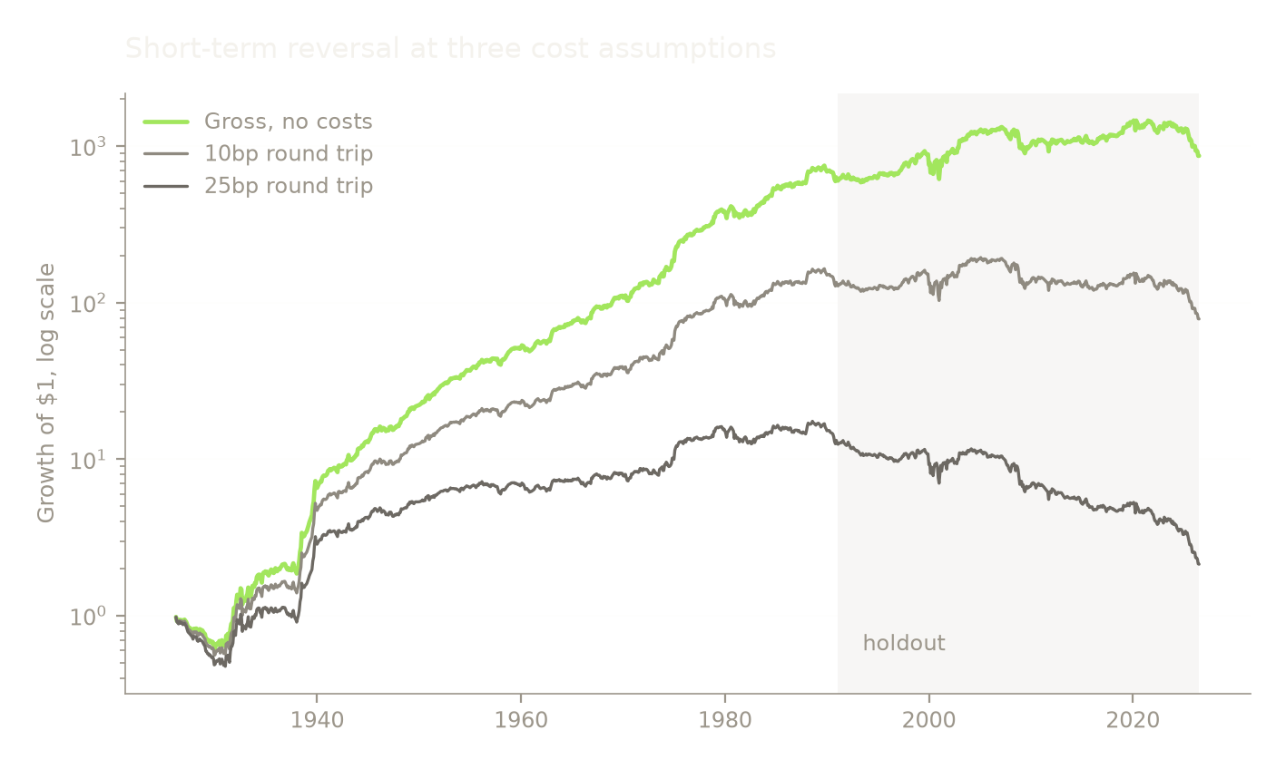
The three lines are the same strategy. Only the cost assumption differs. Over a century a dollar becomes 868 gross, 79 at 10bp, and 2.13 at 25bp.
The 25bp line is the one to look at. It peaks at 17.47 in July 1988 and has fallen to 2.13 since, so a desk paying a quarter of a percent to turn its book over has lost seven eighths of its money over the last thirty-eight years while the gross factor was still rising.
Nothing about the reversal signal differs between those lines. The distance between them is the whole argument for reading a gross factor return with suspicion when the strategy behind it replaces itself every month.
Code7 lines
# The preregistered cost grid, both periods.

print(f"{'cost bps':>9} {'pre mean%':>11} {'pre t':>8}   {'hold mean%':>11} {'hold t':>8}")
for c in P["cost_grid_bps"]:
    a = mean_t(net_of(rev.loc[PRE], c))
    b = mean_t(net_of(rev.loc[OUT], c))
    print(f"{c:>9} {a[1]:+11.3f} {a[2]:+8.2f}   {b[1]:+11.3f} {b[2]:+8.2f}")
cost bps pre mean% pre t hold mean% hold t
0 +0.884 +6.34 +0.143 +0.97
10 +0.684 +4.91 -0.057 -0.39
25 +0.384 +2.75 -0.357 -2.44
50 -0.116 -0.84 -0.857 -5.86
100 -1.116 -8.02 -1.857 -12.70
At 10bp the holdout is already negative. At 25bp it is negative at t = -2.44, which is significantly negative rather than merely unprofitable. The pre-publication period survives 25bp at t = 2.75 and dies before 50bp.
What broke
Code8 lines
# The decade panel, and the breakeven cost in each.

print(f"{'decade':8} {'n':>4} {'mean%':>8} {'t':>7} {'breakeven bps':>14}")
for start in range(1920, 2030, 10):
    s = rev.loc[f"{start}":f"{start + 9}"]
    if len(s) >= 24:
        n, mu, t, _ = mean_t(s)
        print(f"{start}s   {n:>4} {mu:+8.3f} {t:+7.2f} {breakeven_bps(s):>14.1f}")
decade n mean% t breakeven bps 1920s 47 -0.980 -3.25 -49.0 1930s 120 +2.184 +3.52 109.2 1940s 120 +1.047 +5.83 52.3 1950s 120 +0.718 +5.06 35.9 1960s 120 +0.636 +3.25 31.8 1970s 120 +1.088 +4.15 54.4 1980s 120 +0.537 +2.37 26.9 1990s 120 +0.116 +0.52 5.8 2000s 120 +0.355 +1.04 17.7 2010s 120 +0.313 +1.83 15.7 2020s 78 -0.566 -1.58 -28.3
Code30 lines
fig, ax = plt.subplots(figsize=(8, 4.0))

labels, bes = [], []
for start in range(1920, 2030, 10):
    s = rev.loc[f"{start}":f"{start + 9}"]
    if len(s) >= 24:
        labels.append(f"{start}s")
        bes.append(breakeven_bps(s))

# Accent marks the decades that clear the preregistered 25bp threshold. That
# threshold is the verdict, so it is the only thing the colour should encode.
colors = [style.ACCENT if b > 25 else style.SERIES[2] for b in bes]
ax.bar(labels, bes, color=colors, width=0.64)
ax.axhline(0, color=style.MUTED, lw=0.7)

# The 1920s and 2020s are part-decade stubs. Without the counts the chart
# would present 47 months and 120 months as equally solid.
for i, (lab, b) in enumerate(zip(labels, bes)):
    n = len(rev.loc[f"{lab[:4]}":f"{int(lab[:4]) + 9}"])
    ax.annotate(f"n={n}", (i, 0), textcoords="offset points",
                xytext=(0, -14 if b > 0 else 8), ha="center",
                fontsize=7.5, color=style.MUTED)
ax.axhline(25, color=style.SERIES[1], lw=1.1, ls="--")
ax.annotate("25bp, the preregistered threshold", (len(labels) - 0.4, 25),
            textcoords="offset points", xytext=(0, 6), ha="right",
            fontsize=8.5, color=style.MUTED)
ax.set_ylabel("Breakeven round-trip cost, bps")
ax.set_title("The cost at which reversal stops paying, by decade")
ax.tick_params(axis="x", pad=12)
plt.show()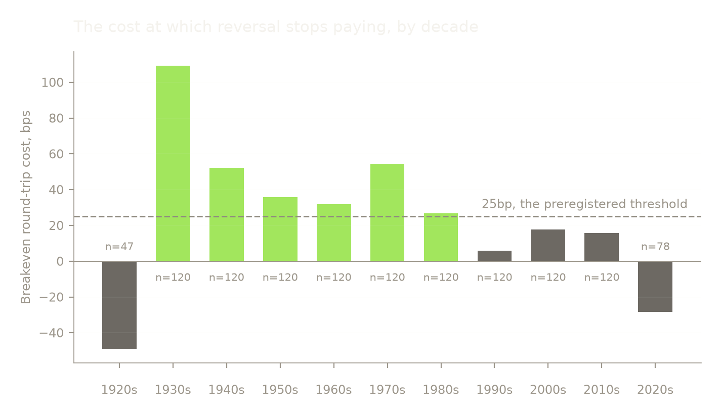
The decline is real but not smooth. Breakeven falls from 109bp in the 1930s to 32bp in the 1960s, rebounds to 54bp in the 1970s, and then drops to 27bp in the 1980s and 6bp in the 1990s. It has stayed in single or low double digits since, and the 2020s are negative, meaning the gross factor itself has lost money this decade.
Every decade after the 1980s sits below the preregistered threshold, and the 1950s, 1960s and 1980s were already between 27 and 36bp, which for a monthly full-turnover strategy was never comfortable. Most of the decline happened before Jegadeesh published in 1990. That fits falling trading costs and rising competition better than it fits a publication event, and this note tests neither explanation.
Code10 lines
# Does the factor just load on the market? Checked in both periods.

joined = pd.DataFrame({"rev": rev}).join(ff[["Mkt-RF", "SMB", "HML"]], how="inner")
print(f"{'period':18} {'alpha%':>8} {'t':>7} {'mkt beta':>10} {'n':>6}")
for label, sl in [("pre-publication", PRE), ("holdout", OUT)]:
    d = joined.loc[sl].dropna()
    fit = sm.OLS(d["rev"], sm.add_constant(d[["Mkt-RF", "SMB", "HML"]])).fit(
        cov_type="HAC", cov_kwds={"maxlags": P["hac_lags"]})
    print(f"{label:18} {fit.params['const']:+8.3f} {fit.tvalues['const']:+7.2f} "
          f"{fit.params['Mkt-RF']:+10.3f} {len(d):>6}")
period alpha% t mkt beta n pre-publication +0.828 +6.34 +0.076 774 holdout -0.077 -0.50 +0.247 426
The decay is not a factor-exposure artefact. Adjusting for market, size and value leaves the same picture: a large, significant alpha before publication and a small, insignificant one after.
Verdict
Do not trade it, and treat its gross Sharpe ratio as close to meaningless. All three preregistered conditions hold.
The gross premium was large and is largely gone: +0.88% a month at t = 6.34 before publication, +0.14% at t = 0.97 since, which is 16% of what it was. That much matches the standard post-publication decay story.
The cost result is the one worth keeping. The breakeven round-trip cost in the holdout is 7.1 basis points. No desk replaces both legs of a long-short book every month at 7bp all-in, so the strategy has not been investable for thirty-five years regardless of what its gross numbers show. Even in the period when it worked, the breakeven was 44bp, which is a thin margin for that turnover and not the free money the gross Sharpe ratio of 0.90 suggests.
The decade panel undercuts a clean publication story. Breakeven costs were already down to 27bp in the 1980s, before Jegadeesh appeared. Whatever removed this premium was probably under way before anyone wrote it down.
The general lesson is the one to carry to any high-turnover factor: a gross factor return is not a strategy return, and for a book that turns over completely every month the gap between them decides everything.
References
French, K. R. (2026). Short-term reversal factor; Fama/French 3 factors. Data library, accessed 2026-08-28. https://mba.tuck.dartmouth.edu/pages/faculty/ken.french/data_library.html
Jegadeesh, N. (1990). Evidence of predictable behavior of security returns. The Journal of Finance 45(3), 881-898. https://onlinelibrary.wiley.com/doi/abs/10.1111/j.1540-6261.1990.tb05110.x
Lehmann, B. N. (1990). Fads, martingales, and market efficiency. The Quarterly Journal of Economics 105(1), 1-28. https://academic.oup.com/qje/article-abstract/105/1/1/1888006
McLean, R. D. and Pontiff, J. (2016). Does academic research destroy stock return predictability? Journal of Finance 71(1), 5-32. https://onlinelibrary.wiley.com/doi/10.1111/jofi.12365
Code6 lines
print(f"python       {sys.version.split()[0]}")
print(f"pandas       {pd.__version__}")
print(f"numpy        {np.__version__}")
print(f"statsmodels  {sm.__version__}")
print(f"seed         {SEED}")
print(f"data as-of   {AS_OF}  (research/data/famafrench/{AS_OF}/)")
python 3.12.13 pandas 3.0.5 numpy 2.5.2 statsmodels 0.15.0 seed 0 data as-of 2026-08-28 (research/data/famafrench/2026-08-28/)