Preregistration — fixed before any data was loaded62 lines
# Frozen before any data is loaded. Every cell below reads from PREREG,
# so no value is typed twice and the plan cannot drift from the code.
#
# Provenance of every parameter.
#
# The Bouman and Jacobsen (2002) paper is behind the AEA paywall and no
# readable copy could be fetched. The AEA page confirms the citation and
# nothing else. Every parameter below that is attributed to them was read
# instead out of Jacobsen and Zhang, "The Halloween Indicator: Everywhere
# and all the time" (SSRN 2154873), which restates the original design:
#   - winter is November through April, summer is May through October
#   - the test is the Halloween dummy regression, r_t = mu + alpha * S_t,
#     where S_t is one in November-April and zero otherwise, on
#     continuously compounded monthly index returns
#   - Bouman and Jacobsen cover January 1970 to August 1998, which is where
#     the holdout starts
#   - Jacobsen and Zhang also run non-overlapping six-month returns, to
#     answer Powell et al.'s objection that a persistent dummy against an
#     autocorrelated series distorts the standard errors. That variant is
#     preregistered here for the same reason.
#
# This is a second-hand reading of a first-hand design, and the note says so.
#
# Mine, not theirs, and named as mine:
#   - cost_bps, hac_lags, the January exclusion cut, and "success".

PREREG = {
    "hypothesis": (
        "In the US market, monthly returns in November through April exceed "
        "those in May through October; the gap is still positive in the "
        "twenty-eight years after Bouman and Jacobsen's sample ends; and a "
        "strategy holding the market only in November through April beats "
        "buy-and-hold on Sharpe ratio in that holdout, net of costs."
    ),
    "universe": (
        "Ken French's US market factor, Mkt-RF plus RF, which is the total "
        "return on all CRSP NYSE, AMEX and NASDAQ common stocks. One series, "
        "not the 37 markets of the original, so this replicates the US result "
        "only. Built from CRSP, so no survivorship bias in universe selection."
    ),
    "start":     "1926-07-31",
    "end":       "2026-06-30",
    "holdout":   "1998-09-30 onwards, touched once in the last cell of Results",
    "rebalance": "twice a year, at the end of April and the end of October",
    "params": {
        "halloween_months": [11, 12, 1, 2, 3, 4],
        "log_returns":      True,
        "hac_lags":         6,
        "cost_bps":         20,
        "six_month_check":  True,
        "drop_january":     True,
    },
    "success": (
        "All three must hold. (a) Over 1926-07 to 1998-08 the Halloween "
        "dummy coefficient is positive with |t| > 2 under Newey-West "
        "standard errors. (b) In the holdout the coefficient is positive. "
        "(c) In the holdout, the switching strategy's Sharpe ratio net of "
        "20bp round-trip costs exceeds buy-and-hold. The January-excluded "
        "regression is reported either way, because the original could not "
        "rule out the January effect for the US."
    ),
}
Setup and imports24 lines
import sys
import warnings

# Library import notices are not findings, and they would otherwise be
# published as output. Silenced before the imports that raise them.
warnings.filterwarnings("ignore")

import numpy as np
import pandas as pd
import statsmodels.api as sm
from scipy import stats
import matplotlib.pyplot as plt

sys.path.append("..")
from lib import style, data

style.use()
SEED = 0
np.random.seed(SEED)

AS_OF = "2026-08-28"          # as-of date of every cached pull in this note
P = PREREG["params"]
MONTH_NAMES = ["Jan", "Feb", "Mar", "Apr", "May", "Jun",
               "Jul", "Aug", "Sep", "Oct", "Nov", "Dec"]
Hypothesis
US stock returns from November through April are higher than from May through October, that gap is still there in the twenty-eight years since the paper that documented it, and a strategy that holds the market only in winter beats buying and holding it.
Bouman and Jacobsen (2002) found winter returns above summer returns in 36 of the 37 markets they looked at. The saying is older than the paper and older than most of the data. This note asks the narrower question a US investor actually faces: on a century of US market returns, is the gap large enough and reliable enough to act on?
The test was fixed before any data was loaded. It is in the first cell, including the three conditions that all had to hold and the holdout that starts where the original sample ends.
Prior work
Bouman, S. and Jacobsen, B. (2002). The Halloween indicator, "Sell in May and go away": another puzzle. American Economic Review 92(5), 1618-1635. The paper being tested. It is behind the AEA paywall and no readable copy could be fetched, so nothing in this note is attributed to its text directly. The citation was confirmed on the AEA article page and the design was read from Jacobsen and Zhang below.
Jacobsen, B. and Zhang, C. Y. The Halloween indicator: everywhere and all the time. Massey University working paper, SSRN 2154873. The source used for every parameter attributed to the original: that winter is November through April and summer is May through October, that Bouman and Jacobsen cover January 1970 to August 1998 across 37 countries, and that the test is a dummy regression on continuously compounded monthly returns. They also run non-overlapping six-month returns to answer Powell et al.'s objection that a persistent dummy against an autocorrelated series distorts standard errors, which is why that check is preregistered here.
This is a second-hand reading of a first-hand design. It is stated here rather than hidden because a parameter taken from a paper nobody opened is the kind of error that produces a plausible number instead of an error message.
McLean, R. D. and Pontiff, J. (2016). Does academic research destroy stock return predictability? Journal of Finance 71(1), 5-32. The reason the holdout starts in September 1998 rather than at a round date.
Data
Ken French's data library, cached on 2026-08-28 under
research/data/famafrench/. One series: the monthly research factors. The
market total return is the market excess return plus the risk-free rate, which
is the return on all CRSP NYSE, AMEX and NASDAQ common stocks. Returns are in
percent.
Built from CRSP, so no survivorship bias enters through universe selection.
Two things this test is not.
It is one market, not 37. Bouman and Jacobsen's headline is a cross-country count. A single-market test has far less statistical power than their design and cannot reproduce their result even in principle. What it can answer is whether a US investor should act, which is the question this note is written to answer.
The sample is longer than theirs, not the same. They cover 1970 to 1998. This covers 1926-07 to 2026-06, so the in-sample period here contains 44 years they did not use. That is deliberate: their sample is short enough that a US result from it alone would be hard to distinguish from noise, and the point of the exercise is to give the effect the most data available.
Code15 lines
ff = data.to_month_end(data.famafrench("F-F_Research_Data_Factors", AS_OF))
ff = ff.loc[PREREG["start"]:PREREG["end"]]

mkt = ff["Mkt-RF"] + ff["RF"]                      # total return, percent
r   = np.log1p(mkt / 100.0) * 100.0                # continuously compounded
S   = pd.Series(np.where(r.index.month.isin(P["halloween_months"]), 1.0, 0.0),
                index=r.index, name="S")

IN  = slice(None, "1998-08-31")                    # their sample ends 1998-08
OUT = slice("1998-09-01", None)                    # holdout, touched once

print(f"factors  {len(ff):6,} rows  {ff.index.min().date()} -> {ff.index.max().date()}")
print(f"winter months {int(S.sum()):,}   summer months {int((1 - S).sum()):,}")
print(f"in sample {len(r.loc[IN]):,} months     holdout {len(r.loc[OUT]):,} months")
print(f"missing values: {int(ff.isna().sum().sum())}")
factors 1,200 rows 1926-07-31 -> 2026-06-30 winter months 600 summer months 600 in sample 866 months holdout 334 months missing values: 0
Method
The regression is the one Jacobsen and Zhang describe: the continuously compounded monthly market return on a constant and a dummy that is one in November through April. The dummy's coefficient is the winter-minus-summer difference in mean monthly return. Standard errors are Newey-West at six lags, because a six-month dummy is autocorrelated by construction.
Three preregistered conditions, all of which had to hold:
- (a) the coefficient is positive with |t| above 2 over 1926-07 to 1998-08
- (b) the coefficient is still positive in the holdout
- (c) in the holdout, holding the market only in winter and Treasury bills otherwise beats buy-and-hold on Sharpe ratio, net of 20bp round trips
Two further checks are preregistered and reported whatever they show. The non-overlapping six-month version answers the objection that a persistent dummy inflates significance. The January-excluded version exists because the original paper could not rule out the January effect as the explanation for the US, and January sits inside the winter window.
Code20 lines
def halloween(y, dummy, lags=P["hac_lags"]):
    """Winter-minus-summer difference in mean monthly return, Newey-West."""
    X = sm.add_constant(pd.DataFrame({"S": dummy}, index=y.index))
    return sm.OLS(y, X).fit(cov_type="HAC", cov_kwds={"maxlags": lags})

def switching(sl, cost_bps=P["cost_bps"]):
    """In the market November-April, in Treasury bills May-October."""
    m  = mkt.loc[sl] / 100.0
    rf = ff["RF"].loc[sl] / 100.0
    weight = pd.Series(np.where(m.index.month.isin(P["halloween_months"]), 1.0, 0.0),
                       index=m.index)
    gross = weight * m + (1 - weight) * rf
    net   = gross - weight.diff().abs().fillna(0) * cost_bps / 10000.0
    return net, m, rf

def sharpe(x, rf):
    return np.sqrt(12) * (x - rf).mean() / (x - rf).std()

def annualised(x):
    return ((1 + x).prod() ** (12 / len(x)) - 1) * 100
Results
Code11 lines
# Criterion (a): is the winter-summer gap significant in sample?

print("winter minus summer, mean monthly return, continuously compounded\n")
print(f"{'period':34} {'n':>5} {'gap%':>8} {'t':>7} {'summer mean%':>13}")
for label, sl in [("in sample  1926-07 to 1998-08", IN),
                  ("full sample 1926-07 to 2026-06", slice(None))]:
    f = halloween(r.loc[sl], S.loc[sl])
    print(f"{label:34} {len(r.loc[sl]):>5} {f.params['S']:+8.3f} "
          f"{f.tvalues['S']:+7.2f} {f.params['const']:+13.3f}")

fit_in = halloween(r.loc[IN], S.loc[IN])
winter minus summer, mean monthly return, continuously compounded period n gap% t summer mean% in sample 1926-07 to 1998-08 866 +0.630 +1.87 +0.519 full sample 1926-07 to 2026-06 1200 +0.588 +2.15 +0.528
Criterion (a) fails. The gap is +0.63% a month in the direction the paper predicts, and its t-statistic is 1.87 against a threshold of 2.
The full-sample number is worth noting precisely because it is tempting. Adding the holdout raises the t-statistic to 2.15, over the line. That number is not a test of anything: it uses the holdout to decide whether the in-sample result was significant, which is the failure the preregistration exists to prevent. The criterion was written against 1926-07 to 1998-08 and that is what it is judged on.
Code16 lines
fig, ax = plt.subplots(figsize=(8, 4.2))

by_month = r.groupby(r.index.month).mean()
order = list(range(1, 13))
colors = [style.ACCENT if mth in P["halloween_months"] else style.SERIES[2]
          for mth in order]

ax.bar([MONTH_NAMES[mth - 1] for mth in order], [by_month[mth] for mth in order],
       color=colors, width=0.66)
ax.axhline(0, color=style.MUTED, lw=0.7)
ax.axhline(r.mean(), color=style.SERIES[1], lw=1.0, ls="--")
ax.annotate("all-month average", (11.4, r.mean()), textcoords="offset points",
            xytext=(0, 5), ha="right", fontsize=8.5, color=style.MUTED)
ax.set_ylabel("Mean monthly return, %")
ax.set_title("Mean return by calendar month, 1926-2026. Winter months in accent.")
plt.show()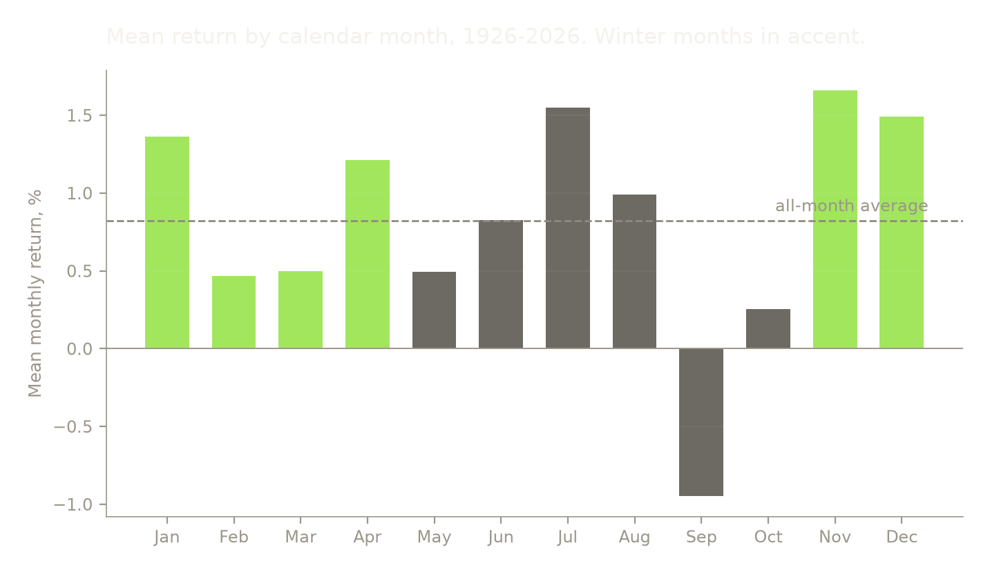
The winter months are mostly above the average and the summer months mostly below, which is the pattern the saying describes. It is not clean. Five of the twelve sit on the wrong side of the line: February and March are winter months below it, and June, July and August are summer months above it. September, at -0.95% a month, is the worst month by a wide margin and carries most of the summer side on its own.
Code21 lines
# The non-overlapping six-month check, preregistered.

def six_month_blocks(x):
    winters, summers = [], []
    for year in range(1927, 2027):
        w = x.loc[f"{year - 1}-11-01":f"{year}-04-30"]
        s = x.loc[f"{year}-05-01":f"{year}-10-31"]
        if len(w) == 6:
            winters.append((year, w.sum()))
        if len(s) == 6:
            summers.append((year, s.sum()))
    return pd.Series(dict(winters)), pd.Series(dict(summers))

win, summ = six_month_blocks(r)
for label, lo, hi in [("in sample", 1927, 1998), ("holdout", 1999, 2026)]:
    w = win[(win.index >= lo) & (win.index <= hi)]
    s = summ[(summ.index >= lo) & (summ.index <= hi)]
    t, pv = stats.ttest_ind(w, s, equal_var=False)
    print(f"{label:10}  winter n={len(w):3d} mean {w.mean():+6.2f}%   "
          f"summer n={len(s):3d} mean {s.mean():+6.2f}%   "
          f"difference {w.mean() - s.mean():+5.2f}   Welch t {t:+.2f}  p {pv:.4f}")
in sample winter n= 72 mean +6.89% summer n= 72 mean +3.27% difference +3.63 Welch t +1.64 p 0.1034 holdout winter n= 28 mean +6.19% summer n= 27 mean +2.72% difference +3.46 Welch t +1.17 p 0.2488
The six-month version, which removes the autocorrelation objection entirely by using one observation per season, is weaker still: t = 1.64 in sample and 1.17 in the holdout. Winter beats summer by roughly 3.5 percentage points per six-month block in both periods, and in neither is that distinguishable from chance.
Code12 lines
# Criteria (b) and (c): the holdout. Evaluated once.

fit_out = halloween(r.loc[OUT], S.loc[OUT])
net_out, mkt_out, rf_out = switching(OUT)

print(f"holdout 1998-09 to 2026-06, n {len(r.loc[OUT])} months\n")
print(f"  winter minus summer gap  {fit_out.params['S']:+.3f}%  t {fit_out.tvalues['S']:+.2f}")
print()
print(f"  switching strategy   annualised {annualised(net_out):+6.2f}%   "
      f"Sharpe {sharpe(net_out, rf_out):+.3f}")
print(f"  buy and hold         annualised {annualised(mkt_out):+6.2f}%   "
      f"Sharpe {sharpe(mkt_out, rf_out):+.3f}")
holdout 1998-09 to 2026-06, n 334 months winter minus summer gap +0.481% t +1.05 switching strategy annualised +7.08% Sharpe +0.483 buy and hold annualised +9.97% Sharpe +0.557
Criterion (b) passes: the gap is still positive out of sample, at +0.48% a month, though at t = 1.05 it is no more significant than it was in sample.
Criterion (c) fails, and it is the one that decides the note. Over the holdout the switching strategy returned 7.08% a year against 9.97% for buying and holding, with a Sharpe ratio of 0.48 against 0.56. Sitting in Treasury bills for half of every year costs more than the seasonal tilt is worth.
Two of the three preregistered conditions fail. The hypothesis is rejected.
Code16 lines
fig, ax = plt.subplots(figsize=(8, 4.3))

net_all, mkt_all, rf_all = switching(slice(None))
ax.plot(net_all.index, (1 + net_all).cumprod(), color=style.ACCENT, lw=1.6,
        label="In the market November-April only")
ax.plot(mkt_all.index, (1 + mkt_all).cumprod(), color=style.SERIES[1], lw=1.2,
        label="Buy and hold")
ax.axvspan(pd.Timestamp("1998-09-30"), net_all.index.max(),
           color=style.SUBTLE, alpha=0.14, lw=0)
ax.annotate("holdout", (pd.Timestamp("2000-06-30"), 2.5),
            fontsize=8.5, color=style.MUTED)
ax.set_yscale("log")
ax.set_ylabel("Growth of $1, log scale")
ax.set_title("Selling in May, net of costs, against holding through")
ax.legend(loc="upper left")
plt.show()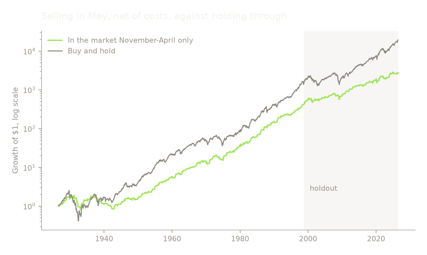
Selling in May was ahead through the Depression, when being out over the summer meant missing part of the crash. It last led in May 1938. Over the eighty-eight years since, it has not been in front in a single month.
A dollar left invested becomes 19,225. The same dollar sold every May becomes 2,795. Avoiding some bad summers cost about seven times the ending wealth.
What broke
Code16 lines
# Every variant tried.

print("January excluded, since it sits inside the winter window\n")
for label, sl in [("in sample", IN), ("holdout", OUT)]:
    rr, ss = r.loc[sl], S.loc[sl]
    keep = rr.index.month != 1
    f = halloween(rr[keep], ss[keep])
    base = halloween(rr, ss)
    print(f"  {label:10} with January  {base.params['S']:+.3f}%  t {base.tvalues['S']:+.2f}"
          f"   without January  {f.params['S']:+.3f}%  t {f.tvalues['S']:+.2f}")

print("\ncost sensitivity in the holdout, strategy Sharpe against buy-and-hold "
      f"{sharpe(mkt_out, rf_out):+.3f}\n")
for c in [0, 20, 50, 100]:
    n, _, rfc = switching(OUT, cost_bps=c)
    print(f"  {c:3d}bp round trip   strategy Sharpe {sharpe(n, rfc):+.3f}")
January excluded, since it sits inside the winter window
in sample with January +0.630% t +1.87 without January +0.501% t +1.46
holdout with January +0.481% t +1.05 without January +0.634% t +1.29
cost sensitivity in the holdout, strategy Sharpe against buy-and-hold +0.557
0bp round trip strategy Sharpe +0.518
20bp round trip strategy Sharpe +0.483
50bp round trip strategy Sharpe +0.431
100bp round trip strategy Sharpe +0.342
Removing January cuts the in-sample gap from +0.63% to +0.50% and the t-statistic from 1.87 to 1.46. So roughly a fifth of the US winter premium is the January effect, which is the explanation the original paper singled out as the one it could not rule out for the US.
The cost grid settles the third criterion. At zero cost the switching strategy still has a lower Sharpe ratio than buy-and-hold, 0.52 against 0.56. The strategy does not lose to transaction costs. It loses because half a year out of the market is expensive whatever the trade costs.
Code9 lines
# Subperiod behaviour, by 25-year block.

print("period       n     gap%       t")
for y0 in [1926, 1951, 1976, 2001]:
    sl = slice(f"{y0}-01-01", f"{y0 + 24}-12-31")
    rr = r.loc[sl]
    if len(rr) > 60:
        f = halloween(rr, S.loc[sl])
        print(f"{y0}-{y0 + 24}  {len(rr):>4}  {f.params['S']:+7.3f}  {f.tvalues['S']:+6.2f}")
period n gap% t 1926-1950 294 -0.290 -0.38 1951-1975 300 +1.160 +2.71 1976-2000 300 +0.979 +2.26 2001-2025 300 +0.499 +1.02
Code16 lines
fig, ax = plt.subplots(figsize=(8, 3.9))

labels, gaps, sig = [], [], []
for y0 in [1926, 1951, 1976, 2001]:
    sl = slice(f"{y0}-01-01", f"{y0 + 24}-12-31")
    f = halloween(r.loc[sl], S.loc[sl])
    labels.append(f"{y0}-{y0 + 24}")
    gaps.append(f.params["S"])
    sig.append(abs(f.tvalues["S"]) > 2)

colors = [style.ACCENT if s else style.SERIES[2] for s in sig]
ax.bar(labels, gaps, color=colors, width=0.55)
ax.axhline(0, color=style.MUTED, lw=0.7)
ax.set_ylabel("Winter minus summer, % per month")
ax.set_title("Blocks reaching |t| > 2 on their own, in accent")
plt.show()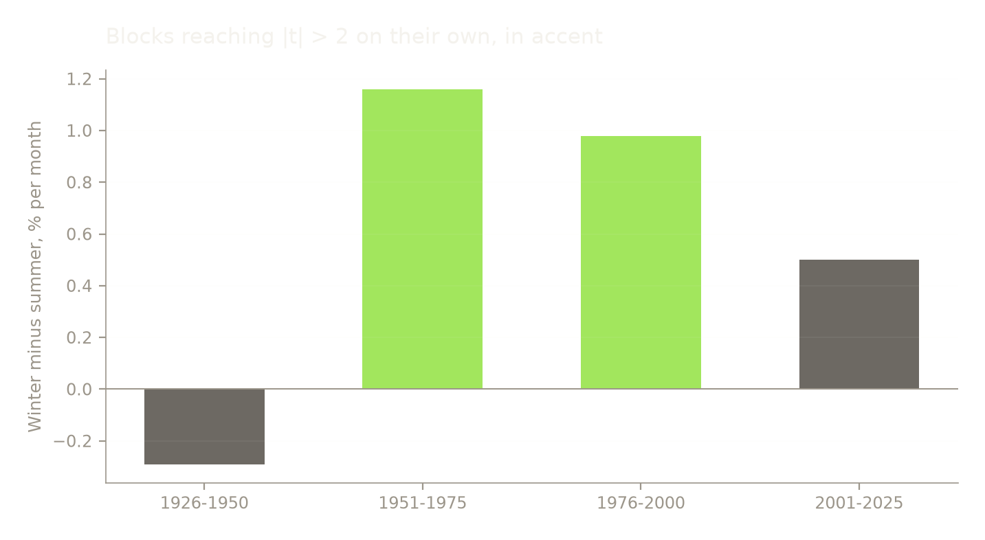
The effect is not stable across the century. The first 25 years run the wrong way at -0.29% a month. The two middle blocks are the whole result, at +1.16% and +0.98%, both clearing t = 2 on their own. The most recent 25 years give +0.50% at t = 1.02.
A seasonal pattern that was absent for the first quarter of the sample, strong for the middle half, and fading in the last quarter is not the kind of thing that supports a rule as blunt as selling every May.
Verdict
Do not trade it. Two of three preregistered conditions fail.
The direction survives everything. Winter beat summer in sample, out of sample, in the six-month blocks, with January removed, and in three of four 25-year blocks. Anyone who says the pattern is not in the data is wrong.
The size is the problem. On the US market alone the gap never reaches conventional significance: t = 1.87 in sample, 1.05 in the holdout, 1.64 and 1.17 on the six-month blocks that remove the autocorrelation objection. And the strategy the saying implies loses to buying and holding, by 2.9 percentage points a year and 0.07 of Sharpe ratio in the holdout, at any cost assumption including zero.
There is no contradiction with Bouman and Jacobsen. Their result is a cross-country count across 37 markets, and this is one market. A pattern can be real in aggregate and too weak to act on in any single place, which appears to be what is happening here.
The practical answer to the question people actually ask: staying invested beat selling in May over the last twenty-eight years, and over the previous seventy as well.
References
Bouman, S. and Jacobsen, B. (2002). The Halloween indicator, "Sell in May and go away": another puzzle. American Economic Review 92(5), 1618-1635. https://www.aeaweb.org/articles?id=10.1257/000282802762024683
French, K. R. (2026). Fama/French 3 factors. Data library, accessed 2026-08-28. https://mba.tuck.dartmouth.edu/pages/faculty/ken.french/data_library.html
Jacobsen, B. and Zhang, C. Y. The Halloween indicator: everywhere and all the time. Massey University working paper. SSRN blocks automated requests, so the copy read for this note is the one below, which carries the SSRN identifier 2154873 on its own first page: https://www.bnains.org/backtest/periode/The_Halloween_Indicator_everywhere_and_all_the_time_-_Ben_Jacobsen_&_Cherry_Y._Zhang.pdf
McLean, R. D. and Pontiff, J. (2016). Does academic research destroy stock return predictability? Journal of Finance 71(1), 5-32. https://onlinelibrary.wiley.com/doi/10.1111/jofi.12365
Code6 lines
print(f"python       {sys.version.split()[0]}")
print(f"pandas       {pd.__version__}")
print(f"numpy        {np.__version__}")
print(f"statsmodels  {sm.__version__}")
print(f"seed         {SEED}")
print(f"data as-of   {AS_OF}  (research/data/famafrench/{AS_OF}/)")
python 3.12.13 pandas 3.0.5 numpy 2.5.2 statsmodels 0.15.0 seed 0 data as-of 2026-08-28 (research/data/famafrench/2026-08-28/)