Preregistration — fixed before any data was loaded91 lines
# Frozen before any data is loaded. Every cell below reads from PREREG,
# so no value is typed twice and the plan cannot drift from the code.
#
# Provenance of every parameter.
#
# From Pontiff & Woodgate (2008), Journal of Finance 63(2), 921-945, abstract
# read on the RePEc page. No readable full text could be fetched: the Wiley
# page returns 403 and no working-paper copy was found. So only the claims
# below are theirs, and no window, threshold, or printed coefficient is
# attributed to them:
#   - "post-1970, share issuance exhibits a strong cross-sectional ability to
#     predict stock returns"
#   - before 1970 they find no statistically significant predictive ability
#     for most holding periods
#
# From Ken French's data library page for Portfolios_Formed_on_NI:
#   - NI for June of year t is the change in the log of split-adjusted shares
#     outstanding from fiscal year-end t-2 to fiscal year-end t-1
#   - portfolios formed each June on NYSE breakpoints; separate portfolios
#     for NI < 0 and NI = 0, then quintiles and deciles
#   - the page does not say whether the quintiles and deciles hold every firm
#     or only the positive-NI firms. The primary spread below is chosen so it
#     means the same thing under either reading: firms that shrank their share
#     count minus the decile that grew it most.
#
# Mine, not theirs, and named as mine:
#   - the use of French's NI measure in place of the paper's own definition,
#     which could not be read
#   - the period boundaries. 1970-01 follows the abstract's "post-1970".
#     The holdout starts in the publication month, April 2008, a date the
#     market could know, rather than at the paper's sample end, which could
#     not be read.
#   - the spread legs, cost_bps, hac_lags, and the decision rule in "success"
#
# French's sample starts in 1963-07, so the pre-1970 period here is 78 months.
# It is reported, but it is too short to test the abstract's pre-1970 claim and
# is not part of the success criterion.

PREREG = {
    "hypothesis": (
        "A value-weighted portfolio long firms that reduced their share count "
        "and short the decile of firms that increased it most earns a positive "
        "Fama-French three-factor alpha after 1970, and that alpha is still "
        "positive and reliably different from zero in the period after "
        "Pontiff and Woodgate was published."
    ),
    "universe": (
        "Ken French Portfolios_Formed_on_NI, value-weighted, built from NYSE, "
        "AMEX and NASDAQ stocks on CRSP, formed each June on net share issues "
        "with NYSE breakpoints. Built from CRSP, so no survivorship bias enters "
        "through universe selection. Includes financials and utilities, as "
        "French's file does."
    ),
    "start":     "1963-07-31",
    "end":       "2026-08-31",
    "holdout":   "2008-04-30 onwards, touched once in the last cell of Results",
    "rebalance": "annual, French forms the portfolios at the end of June",
    "params": {
        "long_leg":       "< 0 ",          # French's column name, trailing space included
        "short_leg":      "Hi 10",
        "insample_start": "1970-01-31",    # abstract: "post-1970"
        "insample_end":   "2008-03-31",    # month before JF 63(2), April 2008
        "cost_bps":       20,              # per leg, charged each July
        "hac_lags":       12,
        "factor_model":   "FF3",           # Mkt-RF, SMB, HML
    },
    "robustness": [
        # Every cut below is reported in What broke, whatever it shows.
        # None of them can change the verdict.
        "Lo 10 minus Hi 10 (the decile spread)",
        "Lo 20 minus Hi 20 (the quintile spread)",
        "equal-weighted version of the primary spread",
        "costs at 0, 20 and 50 bp per leg",
        "five-factor alpha (adds RMW and CMA) in sample and in the holdout, "
        "to see whether the investment factor already absorbs the effect",
        "1963-07 to 1969-12, reported, too short to test",
        "decade-by-decade mean of the primary spread",
    ],
    "success": (
        "Both must hold. (a) Over 1970-01 to 2008-03 the primary spread, net "
        "of costs, has a positive FF3 alpha with Newey-West t > 2. (b) Over "
        "2008-04 to 2026-08 the same alpha is positive with Newey-West t > 2. "
        "If (a) holds and (b) does not, the note reports that the effect is "
        "not reliably present after publication, and says whether the "
        "holdout point estimate is above or below the in-sample one. "
        "If (a) fails, the anomaly was never present in this series and the "
        "holdout question does not arise."
    ),
}

PREREG
{'hypothesis': 'A value-weighted portfolio long firms that reduced their share count and short the decile of firms that increased it most earns a positive Fama-French three-factor alpha after 1970, and that alpha is still positive and reliably different from zero in the period after Pontiff and Woodgate was published.',
'universe': "Ken French Portfolios_Formed_on_NI, value-weighted, built from NYSE, AMEX and NASDAQ stocks on CRSP, formed each June on net share issues with NYSE breakpoints. Built from CRSP, so no survivorship bias enters through universe selection. Includes financials and utilities, as French's file does.",
'start': '1963-07-31',
'end': '2026-08-31',
'holdout': '2008-04-30 onwards, touched once in the last cell of Results',
'rebalance': 'annual, French forms the portfolios at the end of June',
'params': {'long_leg': '< 0 ',
'short_leg': 'Hi 10',
'insample_start': '1970-01-31',
'insample_end': '2008-03-31',
'cost_bps': 20,
'hac_lags': 12,
'factor_model': 'FF3'},
'robustness': ['Lo 10 minus Hi 10 (the decile spread)',
'Lo 20 minus Hi 20 (the quintile spread)',
'equal-weighted version of the primary spread',
'costs at 0, 20 and 50 bp per leg',
'five-factor alpha (adds RMW and CMA) in sample and in the holdout, to see whether the investment factor already absorbs the effect',
'1963-07 to 1969-12, reported, too short to test',
'decade-by-decade mean of the primary spread'],
'success': 'Both must hold. (a) Over 1970-01 to 2008-03 the primary spread, net of costs, has a positive FF3 alpha with Newey-West t > 2. (b) Over 2008-04 to 2026-08 the same alpha is positive with Newey-West t > 2. If (a) holds and (b) does not, the note reports that the effect is not reliably present after publication, and says whether the holdout point estimate is above or below the in-sample one. If (a) fails, the anomaly was never present in this series and the holdout question does not arise.'}Setup and imports23 lines
import sys
import warnings

# Library import notices are not findings, and they would otherwise be
# published as output. Silenced before the imports that raise them.
warnings.filterwarnings("ignore")

import numpy as np
import pandas as pd
import statsmodels.api as sm
import matplotlib.pyplot as plt

sys.path.append("..")
from lib import style, data

style.use()
SEED = 0
np.random.seed(SEED)

AS_OF = "2026-10-14"          # as-of date of every cached pull in this note
P = PREREG["params"]
DECILES = ["Lo 10"] + [f"Dec {i}" for i in range(2, 10)] + ["Hi 10"]
GROUPS = ["< 0 ", "ZERO"] + DECILES
Hypothesis
Firms that buy back their own shares tend to do better afterwards, and firms that issue a lot of new shares tend to do worse. A portfolio long the first group and short the second used to earn a return that the Fama-French three-factor model could not explain. This note tests whether it still does.
Pontiff and Woodgate (2008) reported that after 1970, share issuance predicted returns more reliably than size, book-to-market or momentum. This note checks that claim on Ken French's portfolios sorted on net share issues, then asks what happened in the eighteen years after the paper was published, none of which its authors could have seen.
The test was fixed before any data was loaded. It is in the first cell, including both legs of the spread, the period boundaries, the cost, and the rule that decides the verdict.
Prior work
Pontiff, J. and Woodgate, A. (2008). Share issuance and cross-sectional returns. Journal of Finance 63(2), 921-945. The claim under test. The abstract says that "post-1970, share issuance exhibits a strong cross-sectional ability to predict stock returns", more significant than size, book-to-market or momentum on their own, and that before 1970 there is no significant predictive ability for most holding periods. I could not get a readable copy of the full paper. The publisher's page refuses an automated fetch and I found no working-paper version. So nothing in this note is attributed to the paper beyond those two sentences, and its own issuance measure is not used.
Loughran, T. and Ritter, J. R. (1995). The new issues puzzle. Journal of Finance 50(1), 23-51. The event-study evidence on the issuing side. Over the five years after an offering, investors earned about 5% a year in firms that went public and 7% a year in firms that made a seasoned offering, between 1970 and 1990.
Ikenberry, D., Lakonishok, J. and Vermaelen, T. (1995). Market underreaction to open market share repurchases. Journal of Financial Economics 39(2-3), 181-208. The same on the buyback side: a 12.1% average abnormal four-year return after open market repurchase announcements from 1980 to 1990.
Fama, E. F. and French, K. R. (2008). Dissecting anomalies. Journal of Finance 63(4), 1653-1678. The closest thing to a specification for French's portfolios. They measure net stock issues as the change in the log of split-adjusted shares from fiscal year-end t-2 to t-1, the same definition French's file uses. In their sorts, repurchasers form their own group and positive issuers are split into quintiles. Over 1963 to 2005 the hedge returns were -0.54% to -0.71% a month and more than 4.25 standard errors from zero in every size group. They also found that the negative returns were confined to the most extreme quintile of issuers, and that smaller issues were followed by positive abnormal returns.
McLean, R. D. and Pontiff, J. (2016). Does academic research destroy stock return predictability? Journal of Finance 71(1), 5-32. Across 97 published predictors, returns are 58% lower after publication. It is the reason the holdout starts at the publication date.
Fama, E. F. and French, K. R. (2015). A five-factor asset pricing model. Journal of Financial Economics 116(1), 1-22. The model with an investment factor, CMA. A firm that issues shares is usually growing its assets, so CMA may already carry much of this effect. The five-factor alpha is a preregistered robustness cut for that reason.
Data
Ken French's data library, cached on 2026-10-14 under
research/data/famafrench/. Four series, all monthly and in percent: the
value-weighted and equal-weighted portfolios formed on net share issues, the
three research factors, and the five research factors. The file was built from
the August 2026 CRSP database, so the sample ends in 2026-08.
French builds the portfolios from CRSP himself, so no survivorship bias enters through universe selection. NYSE, AMEX and NASDAQ stocks are included, with financials and utilities.
Four things a reader should hold against this test.
The issuance measure is French's, not Pontiff and Woodgate's. French sorts each June on the change in the log of split-adjusted shares outstanding from fiscal year-end t-2 to t-1. I could not read how the paper defines its own measure, so the note never compares a number here with one from the paper.
French does not say what is inside his deciles. His file has a group for firms that shrank their share count, a group for firms whose count did not change, and then quintiles and deciles. His page does not say whether the deciles hold every firm or only the firms that issued. In Fama and French (2008) only positive issuers are split into quantiles. The primary spread is the repurchaser group minus the top decile, which means the same thing under either reading. The decile-only spread is in What broke.
The default is value-weighted. It is the harder test, since an equal-weighted spread leans on small stocks. The equal-weighted version is preregistered and appears in What broke.
Costs are a rough floor. The portfolios are rebuilt once a year, so the round trip is charged once a year, in July. The cost of borrowing the short leg is not included, and French does not publish holdings that would allow it to be estimated.
Code13 lines
window = slice(PREREG["start"], PREREG["end"])
vw  = data.to_month_end(data.famafrench("Portfolios_Formed_on_NI", AS_OF, table=0)).loc[window]
ew  = data.to_month_end(data.famafrench("Portfolios_Formed_on_NI", AS_OF, table=1)).loc[window]
ff3 = data.to_month_end(data.famafrench("F-F_Research_Data_Factors", AS_OF)).loc[window]
ff5 = data.to_month_end(data.famafrench("F-F_Research_Data_5_Factors_2x3", AS_OF)).loc[window]

for name, d in [("NI, value-weighted", vw), ("NI, equal-weighted", ew),
                ("FF3 factors", ff3), ("FF5 factors", ff5)]:
    print(f"{name:20} {len(d):4} months  {d.index.min().date()} -> {d.index.max().date()}")

used = pd.concat([vw[GROUPS + ["Lo 20", "Hi 20"]], ew[GROUPS + ["Lo 20", "Hi 20"]]], axis=1)
print(f"\nmissing values in the portfolio columns used: {int(used.isna().sum().sum())}")
print(f"French's -99.99 missing-data code in those columns: {int((used <= -99.99).sum().sum())}")
NI, value-weighted 758 months 1963-07-31 -> 2026-08-31 NI, equal-weighted 758 months 1963-07-31 -> 2026-08-31 FF3 factors 758 months 1963-07-31 -> 2026-08-31 FF5 factors 758 months 1963-07-31 -> 2026-08-31 missing values in the portfolio columns used: 0 French's -99.99 missing-data code in those columns: 0
Method
The strategy is long the firms that reduced their share count and short the decile that increased it most, held for a year and rebuilt each June when French rebuilds the portfolios. Both legs are traded once a year, at the preregistered 20bp per leg, charged in July.
Three periods:
- before 1970, 1963-07 to 1969-12, reported only, because 78 months is too short to test anything
- in sample, 1970-01 to 2008-03, from the abstract's "post-1970" to the month before the paper was published
- the holdout, 2008-04 onward, touched once
The test is the intercept of a regression of the net spread on the three Fama-French factors, with Newey-West standard errors at twelve lags. Twelve because the portfolios are held for a year. The spread is a long-short return, so no risk-free rate is subtracted from it.
Code43 lines
FACTORS = {"FF3": ["Mkt-RF", "SMB", "HML"],
           "FF5": ["Mkt-RF", "SMB", "HML", "RMW", "CMA"]}

def spread(long=P["long_leg"], short=P["short_leg"], table=None, cost_bps=P["cost_bps"]):
    """Long minus short, in percent per month, with the annual round trip
    charged in July, the month after French rebuilds the portfolios: out of
    one leg and into the other, so two legs at cost_bps each."""
    table = vw if table is None else table
    gross = table[long] - table[short]
    charge = pd.Series(0.0, index=gross.index)
    charge[gross.index.month == 7] = 2 * cost_bps / 100.0
    return gross - charge

def regress(r, model=P["factor_model"], lags=P["hac_lags"]):
    """Time-series regression on the factors, Newey-West standard errors."""
    f = ff5 if model == "FF5" else ff3
    X = sm.add_constant(f.loc[r.index, FACTORS[model]])
    return sm.OLS(r, X).fit(cov_type="HAC", cov_kwds={"maxlags": lags})

def row(r, model=P["factor_model"]):
    """n, mean and its NW t, alpha and its NW t. All in percent per month."""
    m = sm.OLS(r.values, np.ones(len(r))).fit(cov_type="HAC", cov_kwds={"maxlags": P["hac_lags"]})
    fit = regress(r, model)
    return dict(n=len(r), mean=r.mean(), t_mean=float(m.tvalues[0]),
                alpha=fit.params["const"], t_alpha=fit.tvalues["const"])

def fmt(label, d, w=34):
    return (f"{label:{w}} {d['n']:>4} {d['mean']:+8.3f} {d['t_mean']:+7.2f}"
            f" {d['alpha']:+8.3f} {d['t_alpha']:+7.2f}")

HEADER = f"{'':34} {'n':>4} {'mean%':>8} {'t':>7} {'alpha%':>8} {'t':>7}"

pre70_end = (pd.Timestamp(P["insample_start"]) - pd.offsets.MonthEnd(1)).date().isoformat()
holdout_start = PREREG["holdout"][:10]
PRE70    = slice(PREREG["start"], pre70_end)
INSAMPLE = slice(P["insample_start"], P["insample_end"])
HOLDOUT  = slice(holdout_start, PREREG["end"])

primary = spread()
print(f"primary spread: '{P['long_leg'].strip()}' minus '{P['short_leg']}', value-weighted,"
      f" net of {P['cost_bps']}bp per leg each July")
print(f"in sample  {P['insample_start']} -> {P['insample_end']}")
print(f"holdout    {holdout_start} -> {PREREG['end']}")
primary spread: '< 0' minus 'Hi 10', value-weighted, net of 20bp per leg each July in sample 1970-01-31 -> 2008-03-31 holdout 2008-04-30 -> 2026-08-31
Results
Criterion (a) asks whether the spread earned a three-factor alpha after 1970 and before the paper was published.
Code14 lines
# Criterion (a): in sample, 1970 to the month before publication.
r = primary.loc[INSAMPLE]
d = row(r)
print("net of costs, % per month, Newey-West t\n")
print(HEADER)
print(fmt("in sample, primary spread", d))

fit = regress(r)
print("\nFF3 loadings of the spread in sample")
for k in FACTORS["FF3"]:
    print(f"  {k:7} {fit.params[k]:+6.2f}  (t {fit.tvalues[k]:+6.2f})")

passed_a = d["alpha"] > 0 and d["t_alpha"] > 2
print(f"\ncriterion (a): alpha > 0 and t > 2  ->  {'PASS' if passed_a else 'FAIL'}")
net of costs, % per month, Newey-West t
n mean% t alpha% t
in sample, primary spread 459 +0.636 +3.65 +0.649 +4.81
FF3 loadings of the spread in sample
Mkt-RF -0.14 (t -3.40)
SMB -0.34 (t -4.61)
HML +0.20 (t +2.86)
criterion (a): alpha > 0 and t > 2 -> PASS
It did. The alpha is 0.65% a month at t = 4.81, well clear of the threshold.
The loadings say what kind of portfolio this is. It has a slightly negative market beta and a negative size loading, so the repurchasers it holds are larger than the issuers it shorts. The positive HML loading means the repurchasers are cheaper on book-to-market. The alpha is what is left after all three are accounted for.
The chart below shows where the alpha comes from, group by group, in the same period.
Code26 lines
def group_alphas(sl, table=None):
    table = vw if table is None else table
    out = {}
    for g in GROUPS:
        ex = (table[g] - ff3["RF"]).loc[sl]
        fit = regress(ex)
        out[g] = (fit.params["const"], fit.bse["const"])
    return pd.DataFrame(out, index=["alpha", "se"]).T

ga = group_alphas(INSAMPLE)
labels = ["< 0", "0"] + [str(i) for i in range(1, 11)]
x = np.arange(len(GROUPS))
legs = {P["long_leg"], P["short_leg"]}
colors = [style.ACCENT if g in legs else style.SERIES[2] for g in GROUPS]

fig, ax = plt.subplots(figsize=(8, 4.4))
ax.bar(x, ga["alpha"], color=colors, width=0.7)
ax.axvline(1.5, color=style.MUTED, lw=0.5, alpha=0.5)
ax.errorbar(x, ga["alpha"], yerr=2 * ga["se"], fmt="none", ecolor=style.MUTED, lw=0.8, capsize=2)
ax.axhline(0, color=style.MUTED, lw=0.7)
ax.set_xticks(x, labels)
ax.set_xlabel("Net share issues: repurchased (< 0), unchanged (0), then deciles 1 to 10")
ax.set_ylabel("FF3 alpha, % per month")
ax.set_title(f"In sample, {P['insample_start'][:7]} to {P['insample_end'][:7]}: "
             "alpha by issuance group, value-weighted, ±2 s.e.")
plt.show()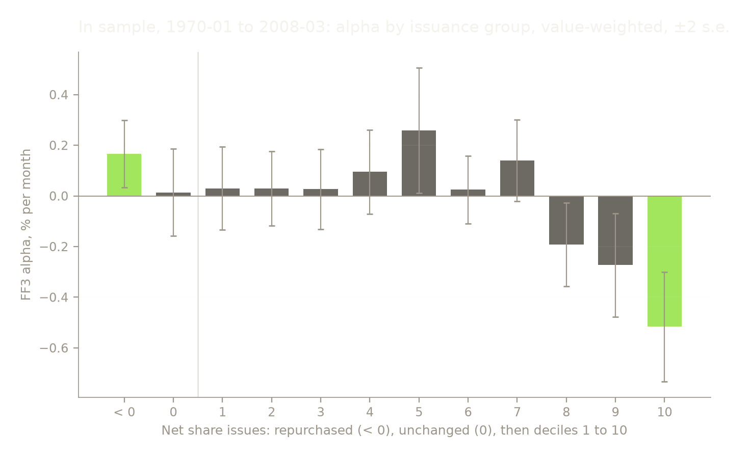
Most of the in-sample spread comes from the issuing side. Deciles 8, 9 and 10 all have negative alphas more than two standard errors from zero, and the top decile is the largest at about -0.5% a month. The repurchasers are positive, and the groups in between are close to zero with one exception in decile 5. This is the same shape Fama and French (2008) describe: the effect sits at the extremes.
Criterion (b) is the holdout, from the month the paper was published to the end of the data. The next cell is the only place it is evaluated.
Code12 lines
# Criterion (b): the holdout. This cell is the only place it is evaluated.
d_in  = row(primary.loc[INSAMPLE])
d_out = row(primary.loc[HOLDOUT])
print("net of costs, % per month, Newey-West t\n")
print(HEADER)
print(fmt("in sample", d_in))
print(fmt("holdout", d_out))

passed_b = d_out["alpha"] > 0 and d_out["t_alpha"] > 2
print(f"\ncriterion (a)  {'PASS' if passed_a else 'FAIL'}")
print(f"criterion (b)  {'PASS' if passed_b else 'FAIL'}")
print(f"holdout alpha is {d_out['alpha'] / d_in['alpha']:.0%} of the in-sample alpha")
net of costs, % per month, Newey-West t
n mean% t alpha% t
in sample 459 +0.636 +3.65 +0.649 +4.81
holdout 221 +0.425 +1.59 +0.613 +2.54
criterion (a) PASS
criterion (b) PASS
holdout alpha is 94% of the in-sample alpha
What broke
Both criteria pass. The holdout alpha is 0.61% a month at t = 2.54, which is 94% of the in-sample alpha. None of the seven earlier notes in this series found a published anomaly that kept a reliable return in its holdout.
The raw mean is a different number. It is 0.43% a month in the holdout at t = 1.59. The spread has a negative market beta, and the market rose through most of the holdout, so the factor adjustment adds return back. Someone who held the spread without hedging the market would have seen the raw number, which is not distinguishable from zero.
Every preregistered cut, in sample and in the holdout. None of them can change the verdict, and all of them are shown.
Code20 lines
VARIANTS = [
    (f"primary, {P['cost_bps']}bp",       lambda: spread(),                                "FF3"),
    ("primary, 0bp",                       lambda: spread(cost_bps=0),                      "FF3"),
    ("primary, 50bp",                      lambda: spread(cost_bps=50),                     "FF3"),
    ("Lo 10 minus Hi 10",                  lambda: spread("Lo 10", "Hi 10"),                "FF3"),
    ("Lo 20 minus Hi 20",                  lambda: spread("Lo 20", "Hi 20"),                "FF3"),
    ("primary, equal-weighted",            lambda: spread(table=ew),                        "FF3"),
    ("primary, five-factor alpha",         lambda: spread(),                                "FF5"),
]

print(f"{'':30} {'in sample':>18} {'holdout':>18}")
print(f"{'variant':30} {'alpha%':>9} {'t':>7}  {'alpha%':>9} {'t':>7}")
for label, f, model in VARIANTS:
    s = f()
    a, b = row(s.loc[INSAMPLE], model), row(s.loc[HOLDOUT], model)
    print(f"{label:30} {a['alpha']:+9.3f} {a['t_alpha']:+7.2f}  {b['alpha']:+9.3f} {b['t_alpha']:+7.2f}")

d = row(primary.loc[PRE70])
print(f"\nbefore 1970, primary spread, {PREREG['start'][:7]} to {pre70_end[:7]}:"
      f" {d['n']} months, alpha {d['alpha']:+.3f}, t {d['t_alpha']:+.2f}")
in sample holdout variant alpha% t alpha% t primary, 20bp +0.649 +4.81 +0.613 +2.54 primary, 0bp +0.683 +5.07 +0.644 +2.66 primary, 50bp +0.597 +4.42 +0.566 +2.35 Lo 10 minus Hi 10 +0.512 +3.60 +0.483 +1.68 Lo 20 minus Hi 20 +0.382 +3.05 +0.241 +1.01 primary, equal-weighted +0.887 +6.56 +1.318 +4.97 primary, five-factor alpha +0.384 +2.98 +0.355 +1.72 before 1970, primary spread, 1963-07 to 1969-12: 78 months, alpha +0.446, t +2.25
Costs barely matter. Moving from 0 to 50bp per leg takes the holdout alpha from 0.64% to 0.57% a month. A strategy that trades once a year is not decided by its trading cost.
The choice of legs matters a lot. Replacing the repurchasers with the lowest decile drops the holdout t to 1.68. The quintile spread drops it to 1.01. The result depends on going long firms that actually reduced their share count, not firms that merely issued little.
Equal-weighting makes it much stronger. The holdout alpha is 1.32% a month at t = 4.97, more than twice the value-weighted number. The effect is larger in small stocks, which also cost more to trade and to borrow than this note charges.
The five-factor model takes away about 40% of it. The alpha falls from 0.65% to 0.38% in sample and from 0.61% to 0.36% in the holdout, where its t is 1.72. By the preregistered threshold, the five-factor version would not pass in the holdout.
Before 1970 the alpha is positive, at t = 2.25. Pontiff and Woodgate's abstract reports no significant predictability before 1970, but their early sample is not described in the abstract and is likely much longer than these 78 months. The two are not compared.
The five-factor loadings show where the 40% went.
Code7 lines
fit5 = {name: regress(primary.loc[sl], "FF5") for name, sl in [("in sample", INSAMPLE), ("holdout", HOLDOUT)]}
print("FF5 loadings of the primary spread\n")
print(f"{'':8} {'in sample':>16} {'holdout':>16}")
for k in ["const"] + FACTORS["FF5"]:
    a, b = fit5["in sample"], fit5["holdout"]
    name = "alpha" if k == "const" else k
    print(f"{name:8} {a.params[k]:+7.2f} (t {a.tvalues[k]:+5.1f}) {b.params[k]:+7.2f} (t {b.tvalues[k]:+5.1f})")
FF5 loadings of the primary spread
in sample holdout
alpha +0.38 (t +3.0) +0.36 (t +1.7)
Mkt-RF -0.06 (t -1.7) -0.11 (t -2.6)
SMB -0.27 (t -3.7) -0.42 (t -5.1)
HML -0.11 (t -1.8) +0.03 (t +0.5)
RMW +0.35 (t +5.0) +0.72 (t +5.6)
CMA +0.70 (t +8.1) +0.42 (t +5.3)
The spread loads heavily on CMA in both periods, at 0.70 in sample and 0.42 in the holdout, and on RMW, at 0.35 and 0.72. Repurchasers tend to be firms that invest conservatively and are profitable. Heavy issuers tend to be the opposite. Once the model contains factors for both, the HML loading falls close to zero and the alpha shrinks. Since 2008 the profitability loading has doubled, so more of the spread now looks like a bet on profitable firms than it did before.
By decade:
Code6 lines
decade = (primary.index.year // 10) * 10
print("primary spread by decade, net, % per month\n")
print(HEADER)
for dec_start, r in primary.groupby(decade):
    lab = f"{r.index.min():%Y-%m} to {r.index.max():%Y-%m}"
    print(fmt(lab, row(r), w=34))
primary spread by decade, net, % per month
n mean% t alpha% t
1963-07 to 1969-12 78 +0.124 +0.39 +0.446 +2.25
1970-01 to 1979-12 120 +0.592 +1.59 +0.557 +2.10
1980-01 to 1989-12 120 +0.760 +3.06 +0.724 +4.02
1990-01 to 1999-12 120 +0.462 +1.89 +0.619 +2.75
2000-01 to 2009-12 120 +0.745 +1.68 +0.525 +2.61
2010-01 to 2019-12 120 +0.343 +1.10 +0.616 +1.73
2020-01 to 2026-08 80 +0.469 +0.95 +0.400 +1.05
The alpha is positive in every decade, including the short 1960s and the partial 2020s. It clears t = 2 in each decade from the 1970s through the 2000s, then falls to 1.73 in the 2010s and 1.05 in the 2020s. The point estimate in the 2010s, 0.62% a month, is in line with the earlier decades. The falling t comes from a noisier spread, not a smaller one.
The raw mean clears t = 2 in only one decade, the 1980s.
Code10 lines
cum = primary.cumsum()
fig, ax = plt.subplots(figsize=(8, 4.4))
ax.axvline(pd.Timestamp(holdout_start), color=style.MUTED, lw=0.9, ls="--")
ax.plot(cum.index, cum.values, color=style.ACCENT, lw=1.6)
ax.axhline(0, color=style.MUTED, lw=0.7)
ax.text(pd.Timestamp(holdout_start), ax.get_ylim()[1], "  holdout starts, April 2008", va="top", color=style.MUTED)
ax.set_ylabel("Cumulative net return, sum of monthly %")
ax.set_title("Repurchasers minus heaviest issuers, value-weighted, net of costs")
style.check_points(ax)
plt.show()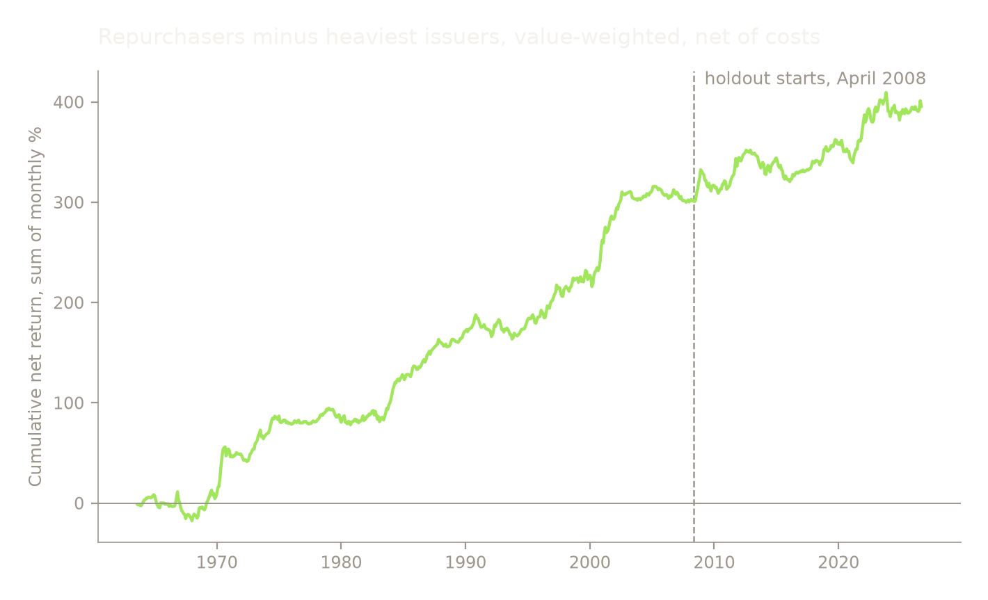
The spread has long flat periods: the second half of the 1970s, 2003 to 2008, and roughly 2013 to 2016. Each lasted years. Someone holding this spread would have spent a large share of the last fifty years without any gain from it.
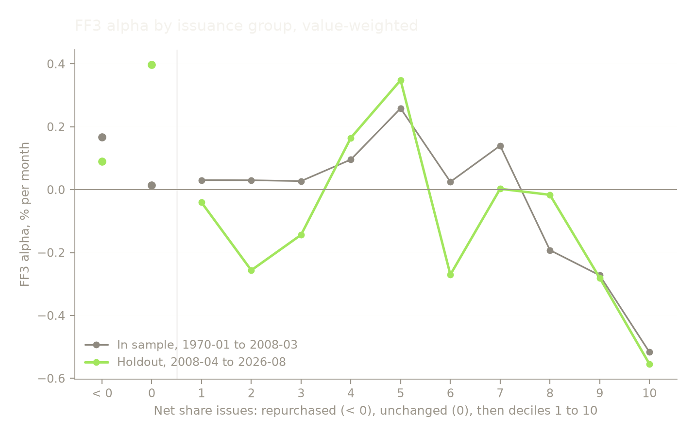
The last chart repeats the group-by-group alphas from Results and adds the holdout.
Code23 lines
gi = group_alphas(INSAMPLE)
gh = group_alphas(HOLDOUT)
print("FF3 alpha by group, value-weighted, % per month (alpha / s.e. in brackets)\n")
print(f"{'group':6} {'in sample':>18} {'holdout':>18}")
for g, lab in zip(GROUPS, labels):
    a, b = gi.loc[g], gh.loc[g]
    print(f"{lab:6} {a['alpha']:+8.3f} ({a['alpha']/a['se']:+5.2f})  {b['alpha']:+8.3f} ({b['alpha']/b['se']:+5.2f})")
fig, ax = plt.subplots(figsize=(8, 4.4))
# Lines join the ten deciles only. Repurchased and unchanged are separate
# groups, not points on the same scale, so they are drawn as markers alone.
dec = x[2:]
for g, color, lw, lab in [(gi, style.SERIES[1], 1.2, f"In sample, {P['insample_start'][:7]} to {P['insample_end'][:7]}"),
                          (gh, style.ACCENT, 1.8, f"Holdout, {holdout_start[:7]} to {PREREG['end'][:7]}")]:
    ax.plot(dec, g["alpha"].iloc[2:], color=color, lw=lw, marker="o", ms=4, label=lab)
    ax.plot(x[:2], g["alpha"].iloc[:2], color=color, lw=0, marker="o", ms=5)
ax.axvline(1.5, color=style.MUTED, lw=0.5, alpha=0.5)
ax.axhline(0, color=style.MUTED, lw=0.7)
ax.set_xticks(x, labels)
ax.set_xlabel("Net share issues: repurchased (< 0), unchanged (0), then deciles 1 to 10")
ax.set_ylabel("FF3 alpha, % per month")
ax.set_title("FF3 alpha by issuance group, value-weighted")
ax.legend(loc="lower left")
plt.show()
FF3 alpha by group, value-weighted, % per month (alpha / s.e. in brackets) group in sample holdout < 0 +0.166 (+2.49) +0.089 (+2.14) 0 +0.014 (+0.16) +0.397 (+2.44) 1 +0.030 (+0.37) -0.041 (-0.18) 2 +0.030 (+0.41) -0.256 (-1.87) 3 +0.027 (+0.34) -0.144 (-1.19) 4 +0.096 (+1.15) +0.165 (+0.90) 5 +0.259 (+2.09) +0.348 (+1.22) 6 +0.025 (+0.37) -0.270 (-1.25) 7 +0.140 (+1.73) +0.003 (+0.01) 8 -0.192 (-2.33) -0.016 (-0.10) 9 -0.273 (-2.67) -0.281 (-1.28) 10 -0.517 (-4.78) -0.555 (-2.60)
Verdict
The anomaly passes, and the result is narrower than the headline. Both preregistered criteria hold. Pontiff and Woodgate's claim replicates on French's portfolios after 1970, and in the eighteen years since the paper was published the three-factor alpha is 0.61% a month at t = 2.54, almost all of what it was.
Three findings limit what that means in practice.
The holdout alpha is almost all on the short side. In the chart above, the top issuance decile has a holdout alpha of -0.56% a month, about the same as before. The repurchasers fell from 0.17% to 0.09%. The rest of the deciles moved around without a pattern. Over 85% of the holdout spread comes from shorting the heaviest issuers, and the cost of borrowing those shares is not in this test. The unchanged-share group earned 0.40% a month in the holdout, at t = 2.44, against 0.01% before. I have no explanation for that, and it is not part of the test.
It is mostly a profitability and investment tilt. The five-factor model explains about 40% of the alpha in both periods, and what remains in the holdout has a t of 1.72. If you already hold profitability and investment factors, this spread adds little that can be measured with eighteen years of data.
The raw return is not significant. Without hedging the market, the spread returned 0.43% a month in the holdout at t = 1.59, with flat periods lasting several years.
So: the signal is real and it survived publication, which none of the seven earlier notes in this series could say. As a reason to avoid stocks that are issuing heavily, the evidence here supports it. As a standalone long-short trade, the verdict is undecided. The return depends on a short leg whose borrowing cost is not measured here, and most of it can be had from two factors that are already widely held.
References
Fama, E. F. and French, K. R. (2008). Dissecting anomalies. Journal of Finance 63(4), 1653-1678. https://ideas.repec.org/a/bla/jfinan/v63y2008i4p1653-1678.html The copy read for this note, and the source of the sort description above: https://www.johnhcochrane.com/s/fama_french_dissecting_anomalies_JF.pdf
Fama, E. F. and French, K. R. (2015). A five-factor asset pricing model. Journal of Financial Economics 116(1), 1-22. https://ideas.repec.org/a/eee/jfinec/v116y2015i1p1-22.html
French, K. R. (2026). Portfolios formed on net share issues; Fama/French 3 factors; Fama/French 5 factors (2x3). Data library, accessed 2026-10-14. https://mba.tuck.dartmouth.edu/pages/faculty/ken.french/data_library.html Construction of the net share issues portfolios: https://mba.tuck.dartmouth.edu/pages/faculty/ken.french/Data_Library/det_port_form_NI.html
Ikenberry, D., Lakonishok, J. and Vermaelen, T. (1995). Market underreaction to open market share repurchases. Journal of Financial Economics 39(2-3), 181-208. https://ideas.repec.org/a/eee/jfinec/v39y1995i2-3p181-208.html
Loughran, T. and Ritter, J. R. (1995). The new issues puzzle. Journal of Finance 50(1), 23-51. https://ideas.repec.org/a/bla/jfinan/v50y1995i1p23-51.html
McLean, R. D. and Pontiff, J. (2016). Does academic research destroy stock return predictability? Journal of Finance 71(1), 5-32. https://onlinelibrary.wiley.com/doi/10.1111/jofi.12365 The publisher's page refuses an automated fetch. The copy read for this note: https://www.gwern.net/doc/economics/2016-mclean.pdf
Pontiff, J. and Woodgate, A. (2008). Share issuance and cross-sectional returns. Journal of Finance 63(2), 921-945. https://ideas.repec.org/a/bla/jfinan/v63y2008i2p921-945.html Only the abstract on this page was read. No readable copy of the full paper could be fetched.
Code10 lines
# What makes this note reproducible after an upstream source updates.
import matplotlib, statsmodels
print(f"python       {sys.version.split()[0]}")
print(f"pandas       {pd.__version__}")
print(f"numpy        {np.__version__}")
print(f"statsmodels  {statsmodels.__version__}")
print(f"matplotlib   {matplotlib.__version__}")
print(f"seed         {SEED}")
print(f"data as-of   famafrench {AS_OF}  (Portfolios_Formed_on_NI t0 and t1,"
      " F-F_Research_Data_Factors, F-F_Research_Data_5_Factors_2x3)")
python 3.12.10 pandas 3.0.5 numpy 2.5.2 statsmodels 0.15.0 matplotlib 3.11.1 seed 0 data as-of famafrench 2026-10-14 (Portfolios_Formed_on_NI t0 and t1, F-F_Research_Data_Factors, F-F_Research_Data_5_Factors_2x3)