Preregistration — fixed before any data was loaded45 lines
# Frozen before any data is loaded. Every cell below reads from PREREG,
# so no value is typed twice and the plan cannot drift from the code.
#
# The state definitions are Daniel & Moskowitz's, not ours. Taken from the
# published paper, JFE 122(2), 221-247, Eq. (4) and Table 5.

PREREG = {
    "hypothesis": (
        "Momentum returns are lower following a bear market combined with high "
        "market variance, and an on/off exposure filter built only on lagged "
        "market data improves the risk-adjusted return of the momentum factor "
        "out of sample."
    ),
    "universe": (
        "Ken French US momentum factor (Mom) and market factor (Mkt-RF, RF), "
        "built from all CRSP US common stocks. French constructs the portfolios, "
        "so no survivorship bias enters through universe choice. Mom is the "
        "6-portfolio (2 size x 3 prior) factor, NOT the decile winner-minus-loser "
        "series Daniel & Moskowitz use. Related, not identical."
    ),
    "start":            "1927-07",
    "end":              "2026-06",
    "first_test_month": "1929-07",   # 24 months of burn-in for the bear indicator
    "holdout": (
        "2013-04 to 2026-06 - everything after the paper's sample end of 2013-03. "
        "Evaluated once, in the last cell of Results."
    ),
    "rebalance": "monthly; state read at the end of month t-1, applied in month t",
    "params": {
        "bear_lookback_months": 24,     # D&M: cumulative market return < 0
        "var_window_days":      126,    # D&M: variance of daily market excess returns
        "vol_threshold":  "expanding median of sigma2_m, min 120 months of history",
        "panic_rule":     "bear == 1 AND sigma2_m > expanding median",
        "weight_normal":  1.0,
        "weight_panic":   0.0,
        "switch_cost_bps": 20,          # charged on notional at each state change
    },
    "success": (
        "BOTH must hold. (a) In sample 1929-07 to 2013-03, the coefficient on the "
        "bear x variance interaction term in the D&M Eq. (4) regression is negative "
        "with t < -2.0. (b) In the holdout 2013-04 to 2026-06, the filtered "
        "strategy's annualised Sharpe exceeds unfiltered momentum's, net of "
        "switching costs. Either one failing is a negative result."
    ),
}
Setup and imports23 lines
import sys
import warnings

# Library import notices are not findings, and they would otherwise be
# published as output. Silenced before the imports that raise them.
warnings.filterwarnings("ignore")

import numpy as np
import pandas as pd
import statsmodels.api as sm
from scipy import stats
import matplotlib.pyplot as plt

sys.path.append("..")
from lib import style, data

style.use()
SEED = 0
np.random.seed(SEED)

AS_OF = "2026-08-28"
P = PREREG["params"]
IS_END, OOS_START = "2013-03-31", "2013-04-01"
Hypothesis
Momentum returns are lower following a bear market combined with high market variance, and an exposure filter built only on lagged market data improves the risk-adjusted return of the momentum factor out of sample.
Daniel and Moskowitz (2016) report that momentum crashes are partly forecastable. They happen after market declines, when volatility is high, and they coincide with market rebounds. This note tests that forecasting claim on Ken French's momentum factor, then asks a second question the paper does not: whether the claim is strong enough to act on in the thirteen years after their sample ends.
The entire test was fixed before any data was loaded. It is in the first cell, including the success criterion and the holdout window.
Prior work
Daniel, K. and Moskowitz, T. J. (2016). Momentum crashes. Journal of Financial Economics 122(2), 221-247. The paper this note replicates. The bear market indicator, the 126-day variance estimate, and the regression tested here are their Eq. (4) and Table 5, estimated on 1927:07 to 2013:03.
Barroso, P. and Santa-Clara, P. (2015). Momentum has its moments. Journal of Financial Economics 116(1), 111-120. Reaches a related conclusion by a different route: scaling momentum exposure by its own trailing realised volatility. Not tested here, but it is the closest alternative to the filter below.
McLean, R. D. and Pontiff, J. (2016). Does academic research destroy stock return predictability? Journal of Finance 71(1), 5-32. Relevant to how the holdout should be read. They find published predictors return 58% less after publication, which is the reason the holdout here starts where the paper's sample ends rather than at an arbitrary date.
Data
Ken French's data library, cached on 2026-08-28 under
research/data/famafrench/. Three series: the monthly momentum factor, the
monthly research factors, and the daily research factors. All returns are in
percent.
French builds these portfolios himself from all CRSP US common stocks, so no survivorship bias enters through universe selection. That is the main reason this note uses his data rather than a price vendor.
Four limits on how closely this can match the paper, all of which affect how the result should be read.
The momentum series is not the one the paper uses. French's Mom factor is
built from six value-weighted portfolios, two size groups crossed with three
prior-return groups. Daniel and Moskowitz use a decile winner-minus-loser
portfolio built from CRSP directly. Decile sorts are more extreme than terciles,
so crashes in their series are larger than crashes here. This is a close
replication, not an exact one, and a weaker result here is partly expected for
that reason alone.
The market series is not identical either. The paper uses the CRSP value-weighted index. French's market factor is CRSP-based but separately constructed, so the bear market indicator computed below will not flag exactly the same months theirs does.
The in-sample window starts two years later than the paper's. The bear indicator needs 24 months of history, so the first testable month is 1929-07 rather than the paper's 1927:07. The 1927-1929 period is excluded from every in-sample figure below.
The switching cost is an assumption, not a measurement. Twenty basis points per state change on the full notional is a plausible round-trip for a liquid factor portfolio, but it was chosen in advance rather than estimated. The sensitivity of the result to that choice is reported in What broke.
Code8 lines
mom = data.to_month_end(data.famafrench("F-F_Momentum_Factor", AS_OF))
ff  = data.to_month_end(data.famafrench("F-F_Research_Data_Factors", AS_OF))
ffd = data.to_daily(data.famafrench("F-F_Research_Data_Factors_daily", AS_OF))

print(f"Mom monthly     {len(mom):6,} rows  {mom.index.min().date()} -> {mom.index.max().date()}")
print(f"Factors monthly {len(ff):6,} rows  {ff.index.min().date()} -> {ff.index.max().date()}")
print(f"Factors daily   {len(ffd):6,} rows  {ffd.index.min().date()} -> {ffd.index.max().date()}")
print(f"missing values: {int(mom.isna().sum().sum() + ff.isna().sum().sum() + ffd.isna().sum().sum())}")
Mom monthly 1,194 rows 1927-01-31 -> 2026-06-30 Factors monthly 1,200 rows 1926-07-31 -> 2026-06-30 Factors daily 26,274 rows 1926-07-01 -> 2026-06-30 missing values: 0
Method
Two state variables, both built only from market data known before the month starts.
Bear market. One when the cumulative market return over the prior 24 months is negative, zero otherwise. The paper specifies the CRSP value-weighted index return, which is a total return, so the market factor and the risk-free rate are added back rather than using the excess return.
Market variance. The variance of daily market excess returns over the 126 trading days preceding the start of the month.
Panic. Bear and variance above its expanding median. The threshold is an expanding median rather than a full-sample one on purpose. A full-sample median would let the state at 1950 depend on volatility levels that had not happened yet, which would make every result before the end of the sample untradeable. The expanding version uses only history available at the time, with a 120-month minimum, so the panic classification does not begin until 1939-06.
The regression is the paper's Eq. (4), with Newey-West standard errors at six lags. The filter holds the momentum factor at full weight normally and at zero in a panic state, charging the preregistered switching cost at each change.
Code23 lines
m = ff.join(mom, how="inner")
m["Mkt"] = m["Mkt-RF"] + m["RF"]                       # total return, as the paper specifies
m = m.loc[PREREG["start"]:PREREG["end"]]

cum = (1 + m["Mkt"] / 100).rolling(P["bear_lookback_months"]).apply(np.prod, raw=True) - 1
m["bear"] = (cum.shift(1) < 0).astype(float)
m.loc[cum.shift(1).isna(), "bear"] = np.nan

dvar = ffd["Mkt-RF"].rolling(P["var_window_days"]).var()
m["sigma2"] = dvar.reindex(m.index, method="ffill").shift(1)

m = m.loc[PREREG["first_test_month"]:].dropna(subset=["bear", "sigma2", "Mom"])

med = m["sigma2"].expanding(min_periods=120).median()
m["panic"] = ((m["bear"] == 1) & (m["sigma2"] > med)).astype(float)
m.loc[med.isna(), "panic"] = np.nan

ins, oos = m.loc[:IS_END], m.loc[OOS_START:]
print(f"panel      {len(m):5,} months  {m.index.min().date()} -> {m.index.max().date()}")
print(f"in-sample  {len(ins):5,} months  {ins.index.min().date()} -> {ins.index.max().date()}")
print(f"holdout    {len(oos):5,} months  {oos.index.min().date()} -> {oos.index.max().date()}")
print(f"panic classification begins {m['panic'].first_valid_index().date()}, "
      f"{int(m['panic'].sum())} panic months of {int(m['panic'].notna().sum())}")
panel 1,164 months 1929-07-31 -> 2026-06-30 in-sample 1,005 months 1929-07-31 -> 2013-03-31 holdout 159 months 2013-04-30 -> 2026-06-30 panic classification begins 1939-06-30, 100 panic months of 1045
Results
Code16 lines
# Criterion (a): the bear x variance interaction, in sample only.

def eq4(df, lags=6, hac=True):
    X = pd.DataFrame({"bear": df["bear"], "sigma2": df["sigma2"],
                      "bear_x_sigma2": df["bear"] * df["sigma2"]}, index=df.index)
    mod = sm.OLS(df["Mom"], sm.add_constant(X))
    return mod.fit(cov_type="HAC", cov_kwds={"maxlags": lags}) if hac else mod.fit()

fit = eq4(ins)
table = pd.DataFrame({"coef": fit.params, "t": fit.tvalues}).round(4)
print(table.to_string())

gate_a = (fit.params["bear_x_sigma2"] < 0) and (fit.tvalues["bear_x_sigma2"] < -2.0)
print(f"\ncriterion (a) requires coef < 0 and t < -2.0  ->  "
      f"coef {fit.params['bear_x_sigma2']:+.4f}, t {fit.tvalues['bear_x_sigma2']:+.2f}  ->  "
      f"{'PASS' if gate_a else 'FAIL'}")
coef t const 1.0036 8.7143 bear -0.4003 -0.5857 sigma2 -0.0921 -0.9465 bear_x_sigma2 -0.3688 -1.1456 criterion (a) requires coef < 0 and t < -2.0 -> coef -0.3688, t -1.15 -> FAIL
The interaction runs in the direction the paper predicts, and it is not close to the significance the criterion demanded. On this series the coefficient is negative in every specification tried later, but the standard error is large enough that the sign carries little weight on its own.
Comparing the two states directly tells a different story from the regression.
Code6 lines
p, n = ins.loc[ins.panic == 1, "Mom"], ins.loc[ins.panic == 0, "Mom"]
t, pv = stats.ttest_ind(p, n, equal_var=False)
print(f"in-sample mean momentum return")
print(f"  panic      {p.mean():+7.3f}%   sd {p.std():5.2f}   n {len(p):4d}")
print(f"  non-panic  {n.mean():+7.3f}%   sd {n.std():5.2f}   n {len(n):4d}")
print(f"  Welch t {t:.2f}   p {pv:.4f}")
in-sample mean momentum return panic -0.766% sd 6.52 n 93 non-panic +0.869% sd 3.50 n 793 Welch t -2.38 p 0.0192
The state means differ, and the difference is significant at the 5% level. Panic months average a loss; other months average a gain roughly the size of the unconditional momentum premium. The variance in panic states is nearly double.
So the paper's mechanism is visible in the data. What fails is the specific functional form the criterion was written against: a linear interaction between a binary state and a continuous variance estimate is a demanding specification, and this series does not support it.
Code13 lines
fig, ax = plt.subplots(figsize=(8, 4.2))
cumret = (1 + m["Mom"] / 100).cumprod()
ax.plot(cumret.index, cumret.values, color=style.ACCENT, label="Momentum factor")
for d in m.index[m["panic"] == 1]:
    ax.axvspan(d - pd.Timedelta(days=15), d + pd.Timedelta(days=15),
               color=style.SUBTLE, alpha=0.22, lw=0)
ax.set_yscale("log")
ax.set_ylabel("Growth of $1, log scale")
ax.set_title("Momentum factor and panic states, 1929-2026\nShaded months are panic states")
ax.legend(loc="upper left")
style.check_points(ax)
plt.tight_layout()
plt.show()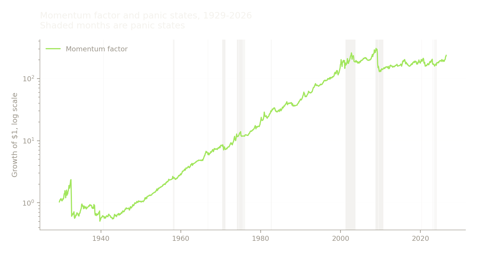
The shaded months cluster where they should: the 1930s, the 1970s, 2002, 2009, and 2023. The largest single drop in the series sits inside a shaded block. Several sharp drops do not.
Code16 lines
fig, ax = plt.subplots(figsize=(8, 4.0))
bins = np.linspace(-40, 30, 50)
# Density, not counts: 93 panic months against 793 makes the shape of the
# panic distribution invisible on a shared count axis.
ax.hist(n, bins=bins, density=True, color=style.SERIES[1], alpha=0.65,
        label=f"Non-panic (n={len(n)})")
ax.hist(p, bins=bins, density=True, color=style.ACCENT, alpha=0.75,
        label=f"Panic (n={len(p)})")
ax.axvline(0, color=style.MUTED, lw=0.6, alpha=0.5)
ax.set_xlim(-40, 25)
ax.set_xlabel("Monthly momentum return, %")
ax.set_ylabel("Share of months in state")
ax.set_title("In-sample monthly momentum returns by state, 1939-2013")
ax.legend()
plt.tight_layout()
plt.show()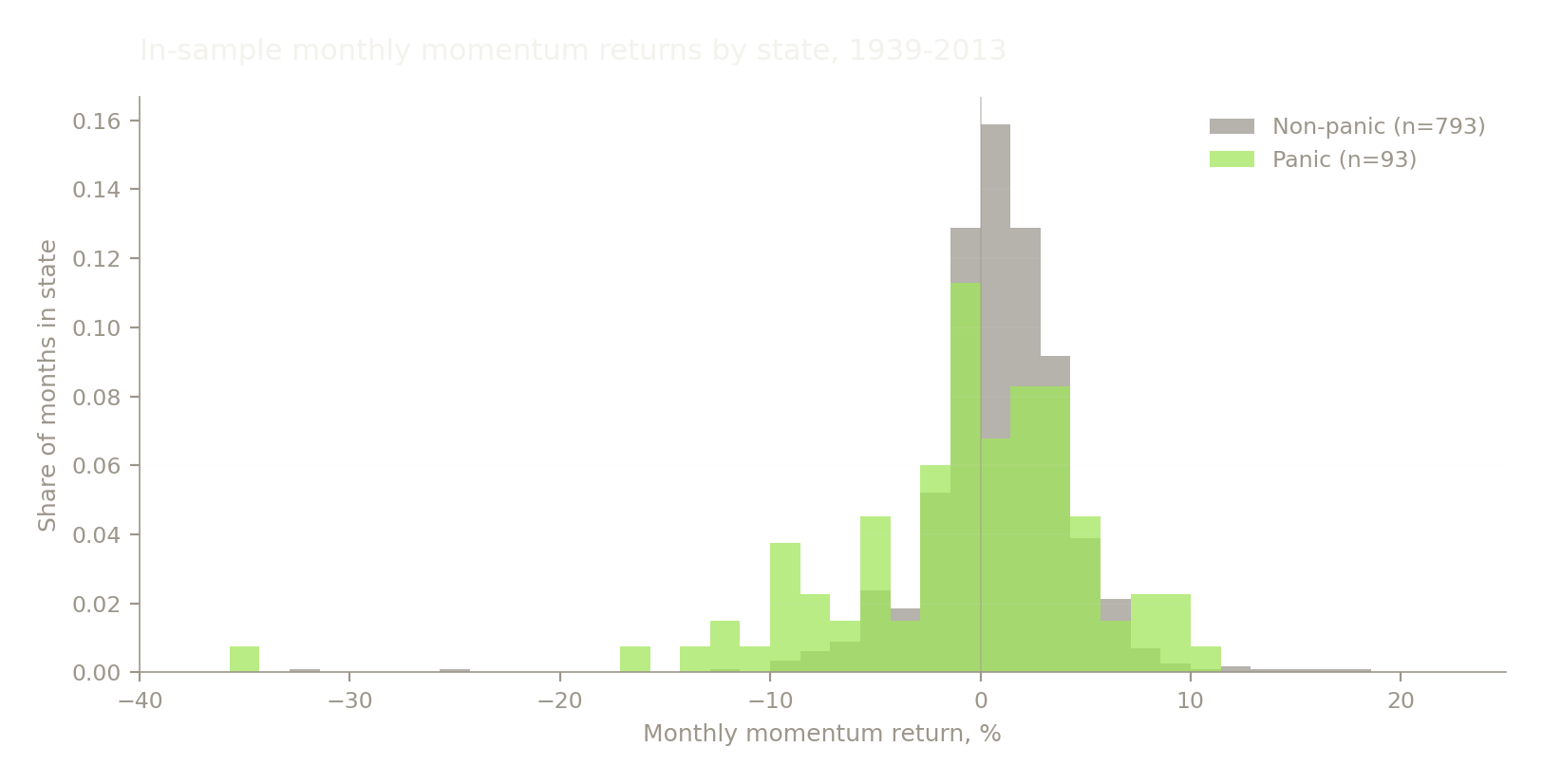
Code23 lines
# Criterion (b): the holdout. Evaluated once.

def sharpe(x):
    return np.sqrt(12) * x.mean() / x.std()

def filtered(df, weight_panic, cost_bps):
    w = pd.Series(np.where(df["panic"] == 1, weight_panic, P["weight_normal"]), index=df.index)
    return w * df["Mom"] - w.diff().abs().fillna(0) * cost_bps / 100.0

hold = oos.dropna(subset=["panic"])
raw = hold["Mom"]
filt = filtered(hold, P["weight_panic"], P["switch_cost_bps"])

print(f"holdout {hold.index.min().date()} -> {hold.index.max().date()}, {len(hold)} months")
print(f"  panic months: {int(hold['panic'].sum())}  "
      f"({', '.join(d.strftime('%Y-%m') for d in hold.index[hold.panic == 1])})")
print(f"  unfiltered  annualised Sharpe {sharpe(raw):.3f}")
print(f"  filtered    annualised Sharpe {sharpe(filt):.3f}")

gate_b = sharpe(filt) > sharpe(raw)
print(f"\ncriterion (b) requires filtered > unfiltered  ->  {'PASS' if gate_b else 'FAIL'}")
print(f"\nOVERALL: (a) {'PASS' if gate_a else 'FAIL'} and (b) {'PASS' if gate_b else 'FAIL'} "
      f"-> {'PASS' if (gate_a and gate_b) else 'FAIL'}")
holdout 2013-04-30 -> 2026-06-30, 159 months panic months: 7 (2020-04, 2023-01, 2023-05, 2023-06, 2023-09, 2023-11, 2023-12) unfiltered annualised Sharpe 0.306 filtered annualised Sharpe 0.500 criterion (b) requires filtered > unfiltered -> PASS OVERALL: (a) FAIL and (b) PASS -> FAIL
Code14 lines
fig, ax = plt.subplots(figsize=(8, 4.0))
ax.plot(hold.index, (1 + raw / 100).cumprod().values, label="Unfiltered momentum")
ax.plot(hold.index, (1 + filt / 100).cumprod().values, label="Filtered")
style.emphasise(ax, index=1)
worst = raw.idxmin()
ax.axvline(worst, color=style.TEXT, lw=0.7, alpha=0.35)
ax.annotate(f"{worst.strftime('%Y-%m')}: {raw.min():.1f}%", xy=(worst, ax.get_ylim()[0]),
            xytext=(8, 14), textcoords="offset points", fontsize=8.5, color=style.MUTED)
ax.set_ylabel("Growth of $1")
ax.set_title("Holdout: 2013-04 to 2026-06")
ax.legend(loc="upper left")
style.check_points(ax)
plt.tight_layout()
plt.show()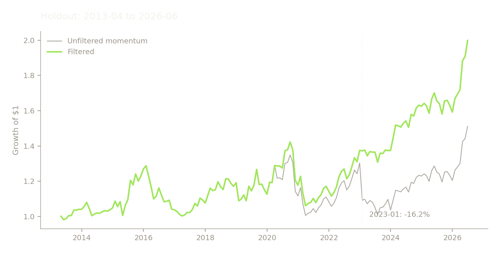
What broke
Three separate weaknesses, reported in the order they matter.
Code14 lines
# Every specification tried, not only the preregistered one.
rows = []
for name, df, lags, hac in [
    ("prereg: HAC(6), 1929-07 to 2013-03", ins, 6, True),
    ("no HAC (plain OLS)",                 ins, 6, False),
    ("HAC(12)",                            ins, 12, True),
    ("HAC(6), from 1940-01 (drop 1930s)",  ins.loc["1940-01":], 6, True),
    ("HAC(6), from 1963-07",               ins.loc["1963-07":], 6, True),
    ("HAC(6), full sample incl. holdout",  m, 6, True),
]:
    f = eq4(df, lags=lags, hac=hac)
    rows.append({"specification": name, "coef": round(f.params["bear_x_sigma2"], 4),
                 "t": round(f.tvalues["bear_x_sigma2"], 2), "months": len(df)})
print(pd.DataFrame(rows).to_string(index=False))
specification coef t months
prereg: HAC(6), 1929-07 to 2013-03 -0.3688 -1.15 1005
no HAC (plain OLS) -0.3688 -1.73 1005
HAC(12) -0.3688 -1.28 1005
HAC(6), from 1940-01 (drop 1930s) -0.6696 -1.70 879
HAC(6), from 1963-07 -0.7550 -1.79 597
HAC(6), full sample incl. holdout -0.3944 -1.25 1164
The sign never flips. The significance never arrives. The strongest reading, t = -1.79 on post-1963 data, still falls short of the threshold set in advance, and choosing it after the fact would not make it a test.
The gap between plain OLS at t = -1.73 and Newey-West at t = -1.15 is worth noting on its own. The result depends materially on how standard errors are computed, which is a sign the estimate is fragile rather than borderline.
Code18 lines
# Every filter variant tried, not only the preregistered one.
ter = m["sigma2"].expanding(min_periods=120).quantile(2 / 3)
variants = {
    "prereg: median threshold, w=0, 20bp": (m["panic"], 0.0, 20),
    "tercile threshold":                   (((m["bear"] == 1) & (m["sigma2"] > ter)).astype(float).where(ter.notna()), 0.0, 20),
    "bear only, variance ignored":         ((m["bear"] == 1).astype(float).where(med.notna()), 0.0, 20),
    "half weight instead of zero":         (m["panic"], 0.5, 20),
    "zero switching cost":                 (m["panic"], 0.0, 0),
    "50bp switching cost":                 (m["panic"], 0.0, 50),
}
base = sharpe(hold["Mom"])
rows = [{"variant": "unfiltered momentum", "sharpe": round(base, 3), "vs raw": "--", "panic months": 0}]
for name, (col, wp, cb) in variants.items():
    h = oos.assign(panic=col.reindex(oos.index)).dropna(subset=["panic"])
    s = sharpe(filtered(h, wp, cb))
    rows.append({"variant": name, "sharpe": round(s, 3), "vs raw": f"{s - base:+.3f}",
                 "panic months": int(h["panic"].sum())})
print(pd.DataFrame(rows).to_string(index=False))
variant sharpe vs raw panic months
unfiltered momentum 0.306 -- 0
prereg: median threshold, w=0, 20bp 0.500 +0.194 7
tercile threshold 0.483 +0.177 4
bear only, variance ignored 0.492 +0.186 8
half weight instead of zero 0.407 +0.101 7
zero switching cost 0.513 +0.207 7
50bp switching cost 0.481 +0.175 7
Code9 lines
# How much of the holdout result is one month?
h2 = hold.drop(index=hold["Mom"].idxmin())
print(f"holdout worst month: {hold['Mom'].idxmin().strftime('%Y-%m')}  "
      f"{hold['Mom'].min():.2f}%   panic flag = {int(hold.loc[hold['Mom'].idxmin(), 'panic'])}")
print(f"\n{'':22} {'with it':>9} {'without':>9}")
print(f"{'unfiltered Sharpe':22} {sharpe(hold['Mom']):9.3f} {sharpe(h2['Mom']):9.3f}")
print(f"{'filtered Sharpe':22} {sharpe(filtered(hold, 0.0, 20)):9.3f} {sharpe(filtered(h2, 0.0, 20)):9.3f}")
print(f"{'gap':22} {sharpe(filtered(hold, 0.0, 20)) - sharpe(hold['Mom']):+9.3f} "
      f"{sharpe(filtered(h2, 0.0, 20)) - sharpe(h2['Mom']):+9.3f}")
holdout worst month: 2023-01 -16.21% panic flag = 1
with it without
unfiltered Sharpe 0.306 0.429
filtered Sharpe 0.500 0.505
gap +0.194 +0.075
The holdout result is one month. January 2023 was flagged as a panic state, momentum lost 16.2% that month, and the filter was out of the market for it. Remove that single observation and the advantage nearly disappears. Seven panic months in thirteen years was never going to support a strong conclusion, and the concentration makes it weaker still. Criterion (b) passed on a technicality.
The filter misses crashes it should catch. Of the five worst in-sample momentum months, three were flagged and two were not, including September 1939 at -31.5%. A filter that catches some crashes and not others is a different proposition from one that catches crashes.
The replication is not exact, and the direction of the mismatch is known. French's momentum factor is built on tercile sorts, the paper's on deciles. Decile portfolios hold more extreme past winners and losers, so their crashes are larger and the state effect on them should be easier to detect. A weaker result here is consistent with the paper being right about decile portfolios and this series being the wrong instrument to test it on. That possibility cannot be separated from the paper being weaker than reported, and this note does not try to.
Verdict
The preregistered test fails. Criterion (a) required the bear-variance interaction to be negative with t below -2.0 in sample. It came in at -1.15. Criterion (b) passed, but on seven observations, and almost entirely on one of them. Both had to hold. They did not.
That is not the same as saying Daniel and Moskowitz are wrong. The state effect is visible here: panic months average a loss where other months average a gain, the difference is significant at the 5% level, and the sign of the interaction is negative in every specification tried. The effect is not strong enough to survive this test on a related but different series. That is a narrower claim than either "it replicates" or "it does not."
Do not trade this filter. Not because the idea is wrong, but because nothing here establishes that it works. A rule that fires seven times in thirteen years and earns its entire out-of-sample advantage in one month is indistinguishable from luck at this sample size, and no amount of favourable-looking Sharpe improvement changes that.
The honest next step is the decile winner-minus-loser series the paper actually uses, built from CRSP. If the effect is real and this note simply used the wrong instrument, that is where it would show up.
References
Barroso, P. and Santa-Clara, P. (2015). Momentum has its moments. Journal of Financial Economics 116(1), 111-120. https://econpapers.repec.org/RePEc:eee:jfinec:v:116:y:2015:i:1:p:111-120
Daniel, K. and Moskowitz, T. J. (2016). Momentum crashes. Journal of Financial Economics 122(2), 221-247. https://www.nber.org/papers/w20439
McLean, R. D. and Pontiff, J. (2016). Does academic research destroy stock return predictability? Journal of Finance 71(1), 5-32. https://onlinelibrary.wiley.com/doi/abs/10.1111/jofi.12365
Data: Kenneth R. French data library, retrieved 2026-08-28. https://mba.tuck.dartmouth.edu/pages/faculty/ken.french/data_library.html
Code6 lines
print(f"python      {sys.version.split()[0]}")
print(f"pandas      {pd.__version__}")
print(f"numpy       {np.__version__}")
print(f"statsmodels {sm.__version__}")
print(f"seed        {SEED}")
print(f"data as-of  Ken French library, {AS_OF}")
python 3.10.9 pandas 2.3.1 numpy 1.23.5 statsmodels 0.13.5 seed 0 data as-of Ken French library, 2026-08-28