Preregistration — fixed before any data was loaded61 lines
# Frozen before any data is loaded. Every cell below reads from PREREG,
# so no value is typed twice and the plan cannot drift from the code.
#
# Provenance of every parameter, because a number attributed to a paper
# nobody opened is a fabricated citation wearing a number.
#
# From Frazzini & Pedersen (2014), JFE 111(1), 1-25, read out of the
# author copy at w4.stern.nyu.edu:
#   - the prediction tested: "the alphas decline almost monotonically from
#     the low-beta to high-beta portfolios" (their Proposition 1, Table III)
#   - the BAB construction: each leg rescaled to a beta of one at formation,
#     long low-beta, short high-beta, self-financing at the risk-free rate
#     (their Eq. 17)
#   - their US sample ends March 2012, which is where the holdout starts
#
# Mine, not theirs, and named as mine:
#   - post_rank_beta_window_months. Frazzini and Pedersen estimate stock
#     betas from a 1-year volatility window and a 5-year correlation window
#     and shrink 0.6 of the way toward 1. That is a stock-level device and
#     the sort here is already done by French, so the rescaling beta is a
#     plain 60-month rolling regression of the decile on the market. Their
#     shrinkage is deliberately not applied.
#   - cost_bps and hac_lags.

PREREG = {
    "hypothesis": (
        "CAPM alphas fall as pre-ranking beta rises across Ken French's "
        "beta-sorted deciles; a beta-neutral portfolio long the low-beta "
        "decile and short the high-beta decile, each rescaled to a beta of "
        "one, earns positive three-factor alpha net of costs; and that "
        "portfolio has a positive Sharpe ratio in the fourteen years after "
        "Frazzini and Pedersen's sample ends."
    ),
    "universe": (
        "Ken French Portfolios_Formed_on_BETA, value-weighted deciles built "
        "from NYSE, AMEX and NASDAQ common stocks on CRSP, sorted each June "
        "on Scholes-Williams betas from the prior 60 months. French builds "
        "the portfolios from CRSP himself, so no survivorship bias enters "
        "through universe selection. The sort is not Frazzini and Pedersen's "
        "beta estimator, which is the main gap between this test and theirs."
    ),
    "start":     "1963-07-31",
    "end":       "2026-06-30",
    "holdout":   "2012-04-30 onwards, touched once in the last cell of Results",
    "rebalance": "monthly, from French's monthly portfolio returns",
    "params": {
        "n_deciles":                    10,
        "post_rank_beta_window_months": 60,
        "post_rank_beta_min_months":    36,
        "cost_bps":                     10,
        "hac_lags":                     6,
    },
    "success": (
        "All three must hold. (a) In sample, the Spearman rank correlation "
        "between decile number and CAPM alpha is negative with p < 0.05. "
        "(b) In sample, the rescaled long-short portfolio has a positive "
        "Fama-French three-factor alpha with |t| > 2 under Newey-West "
        "standard errors, net of 10bp round-trip costs. (c) In the holdout, "
        "that portfolio's net Sharpe ratio is positive."
    ),
}
Setup and imports23 lines
import sys
import warnings

# Library import notices are not findings, and they would otherwise be
# published as output. Silenced before the imports that raise them.
warnings.filterwarnings("ignore")

import numpy as np
import pandas as pd
import statsmodels.api as sm
from scipy import stats
import matplotlib.pyplot as plt

sys.path.append("..")
from lib import style, data

style.use()
SEED = 0
np.random.seed(SEED)

AS_OF = "2026-08-28"          # as-of date of every cached pull in this note
P = PREREG["params"]
DECILES = ["Lo 10"] + [f"Dec {i}" for i in range(2, 10)] + ["Hi 10"]
Hypothesis
CAPM alphas fall as beta rises. A portfolio that is long low-beta stocks levered up to a beta of one, and short high-beta stocks scaled down to a beta of one, earns a positive return that the three-factor model does not explain. That premium is still there in the fourteen years after the paper that described it.
Frazzini and Pedersen (2014) argue that investors who cannot borrow freely bid up high-beta assets instead, which flattens the security market line and leaves a premium for anyone willing to lever a low-beta portfolio. This note tests both halves of that claim on Ken French's beta-sorted deciles, and then asks the question the paper could not: whether the premium survived the fourteen years after their sample ended in March 2012.
The whole test was fixed before any data was loaded. It is in the first cell, including which parameters came from the paper, which are mine, the success criterion, and the holdout.
Prior work
Frazzini, A. and Pedersen, L. H. (2014). Betting against beta. Journal of Financial Economics 111(1), 1-25. The paper this note tests. Their Proposition 1 predicts that alphas decline with beta, and their Table III reports that they "decline almost monotonically from the low-beta to high-beta portfolios". Their BAB factor, Eq. (17), rescales each leg to a beta of one and is self-financing at the risk-free rate. Their US sample runs to March 2012, which is where the holdout here begins.
Black, F., Jensen, M. C. and Scholes, M. (1972). The capital asset pricing model: some empirical tests. In Studies in the Theory of Capital Markets. The original finding that the security market line is too flat for the CAPM. Frazzini and Pedersen's contribution is an explanation for it and a portfolio that harvests it, not the observation itself.
Novy-Marx, R. and Velikov, M. (2022). Betting against betting against beta. Journal of Financial Economics 143(1), 80-106. The strongest published objection: they argue the BAB factor's returns come from its implicit bet on small, illiquid, low-priced stocks and from the non-standard weighting scheme, not from leverage constraints. This note cannot separate those explanations, because French's deciles are value-weighted and fixed, so the weighting objection is untestable here. It is the main reason a positive result below should not be read as confirming the paper's mechanism.
McLean, R. D. and Pontiff, J. (2016). Does academic research destroy stock return predictability? Journal of Finance 71(1), 5-32. They find published predictors return 58% less after publication. That is why the holdout starts where the paper's sample ends rather than at a round date.
Data
Ken French's data library, cached on 2026-08-28 under
research/data/famafrench/. Two series: the monthly beta-sorted portfolios and
the monthly research factors. All returns are in percent.
French builds these portfolios from every CRSP US common stock himself, so no survivorship bias enters through universe selection. That is the reason this note uses his data rather than a price vendor.
Three gaps between this test and the paper, all of which change how the result should be read.
The sort is not their beta. French forms the deciles each June on Scholes-Williams betas estimated from the prior 60 months of returns. Frazzini and Pedersen estimate stock betas from a one-year volatility window and a five-year correlation window on overlapping three-day returns, then shrink the estimate 0.6 of the way toward one, and they re-sort monthly. Their portfolios are also rank-weighted rather than value-weighted. So this is a test of their prediction on a standard beta sort, not a reconstruction of their factor.
Costs are undercounted. The only turnover this note can charge for is the change in the leverage weights, because French publishes portfolio returns and not holdings. The deciles themselves reshuffle each June, and that turnover is invisible here. The cost figures below are therefore a floor, not an estimate. The sensitivity grid in What broke runs to 100bp to show how little it matters either way.
The sample starts in 1963. French's beta-sorted portfolios begin in 1963-07, so this covers 63 years rather than the paper's 1926 start. The 1926-1963 period, which includes the Depression, is absent.
Code15 lines
dec = data.to_month_end(data.famafrench("Portfolios_Formed_on_BETA", AS_OF, table=0))
ff  = data.to_month_end(data.famafrench("F-F_Research_Data_Factors", AS_OF))

m = dec[DECILES].join(ff[["Mkt-RF", "RF", "SMB", "HML"]], how="inner")
m = m.loc[PREREG["start"]:PREREG["end"]]
ex = m[DECILES].sub(m["RF"], axis=0)          # excess returns, percent per month

ins = ex.loc[:"2012-03-31"]                    # paper's sample ends March 2012
oos = ex.loc["2012-04-30":]                    # holdout, touched once at the end

print(f"deciles   {len(dec):6,} rows  {dec.index.min().date()} -> {dec.index.max().date()}")
print(f"factors   {len(ff):6,} rows  {ff.index.min().date()} -> {ff.index.max().date()}")
print(f"merged    {len(m):6,} rows  {m.index.min().date()} -> {m.index.max().date()}")
print(f"in-sample {len(ins):6,} months     holdout {len(oos):,} months")
print(f"missing values in the merged panel: {int(m.isna().sum().sum())}")
deciles 756 rows 1963-07-31 -> 2026-06-30 factors 1,200 rows 1926-07-31 -> 2026-06-30 merged 756 rows 1963-07-31 -> 2026-06-30 in-sample 585 months holdout 171 months missing values in the merged panel: 0
Method
Two tests, matching the paper's two predictions.
Does alpha fall as beta rises? Each decile's excess return is regressed on the market excess return over the in-sample period, with Newey-West standard errors. The rank correlation between decile number and CAPM alpha is the statistic the criterion was written against. A rank correlation is used rather than a slope because the prediction is about ordering, and one extreme decile should not be able to carry the result on its own.
Does the levered spread pay? The portfolio is the paper's Eq. (17) applied at portfolio level: long the low-beta decile scaled by one over its beta, short the high-beta decile scaled by one over its beta, self-financing at the risk-free rate. Each beta comes from a 60-month rolling regression of the decile on the market, shifted by one month so the weight for a given month uses only returns that had already happened. That shift is what keeps the portfolio tradeable rather than a description of the past.
The paper's 0.6 shrinkage toward a beta of one is deliberately not applied. It is a device for noisy single-stock betas, and a decile of hundreds of stocks does not have that problem. Skipping it is my decision, and it is named as mine in the preregistration cell.
Costs are charged on the change in the two leverage weights each month, at the preregistered 10bp round trip.
Code20 lines
def capm(y, x, lags=P["hac_lags"]):
    return sm.OLS(y, sm.add_constant(x)).fit(cov_type="HAC", cov_kwds={"maxlags": lags})

def rolling_beta(y, x, window=P["post_rank_beta_window_months"],
                 min_periods=P["post_rank_beta_min_months"]):
    """Beta of y on x from a trailing window, shifted so month t uses only
    data through t-1. Without the shift the portfolio would be using its own
    contemporaneous return to size itself."""
    cov = y.rolling(window, min_periods=min_periods).cov(x)
    var = x.rolling(window, min_periods=min_periods).var()
    return (cov / var).shift(1)

def bab_factor(ex_panel, mkt, lo="Lo 10", hi="Hi 10", cost_bps=P["cost_bps"]):
    """Frazzini and Pedersen Eq. (17) at portfolio level: each leg rescaled to
    a beta of one, long low, short high, self-financing at the risk-free rate."""
    w_lo = 1.0 / rolling_beta(ex_panel[lo], mkt)
    w_hi = 1.0 / rolling_beta(ex_panel[hi], mkt)
    gross = w_lo * ex_panel[lo] - w_hi * ex_panel[hi]
    turnover = w_lo.diff().abs().fillna(0) + w_hi.diff().abs().fillna(0)
    return gross - turnover * cost_bps / 100.0, w_lo, w_hi, turnover
Results
Code26 lines
# Criterion (a): does alpha decline with beta? In sample only.

mkt_ins = m.loc[ins.index, "Mkt-RF"]
rows = []
for i, col in enumerate(DECILES, start=1):
    fit = capm(ins[col], mkt_ins)
    rows.append({
        "decile": i,
        "beta":   fit.params["Mkt-RF"],
        "mean":   ins[col].mean(),
        "alpha":  fit.params["const"],
        "t":      fit.tvalues["const"],
        "sharpe": np.sqrt(12) * ins[col].mean() / ins[col].std(),
    })
tab = pd.DataFrame(rows)

rho,  pval  = stats.spearmanr(tab["decile"], tab["alpha"])
rho2, pval2 = stats.spearmanr(tab["decile"], tab["sharpe"])

print("1963-07 to 2012-03, value-weighted beta deciles, monthly percent\n")
print(f"{'decile':>6} {'beta':>7} {'mean':>7} {'alpha':>7} {'t':>7} {'sharpe':>7}")
for r in rows:
    print(f"{r['decile']:>6} {r['beta']:7.2f} {r['mean']:7.3f} "
          f"{r['alpha']:+7.3f} {r['t']:+7.2f} {r['sharpe']:7.2f}")
print(f"\nSpearman(decile, alpha)  rho {rho:+.3f}   p {pval:.4f}")
print(f"Spearman(decile, Sharpe) rho {rho2:+.3f}   p {pval2:.4f}")
1963-07 to 2012-03, value-weighted beta deciles, monthly percent
decile beta mean alpha t sharpe
1 0.62 0.484 +0.199 +2.12 0.47
2 0.73 0.441 +0.104 +1.21 0.39
3 0.83 0.499 +0.114 +1.54 0.42
4 0.97 0.599 +0.154 +1.84 0.44
5 1.01 0.494 +0.027 +0.48 0.35
6 1.09 0.564 +0.062 +0.88 0.37
7 1.16 0.486 -0.049 -0.69 0.30
8 1.27 0.578 -0.008 -0.09 0.33
9 1.39 0.622 -0.017 -0.15 0.32
10 1.61 0.618 -0.124 -0.79 0.27
Spearman(decile, alpha) rho -0.903 p 0.0003
Spearman(decile, Sharpe) rho -0.903 p 0.0003
Alpha falls from +0.20% a month in the lowest-beta decile to -0.12% in the highest, and the rank correlation is -0.90 at p = 0.0003. Criterion (a) is met.
The mean column is the more striking one. Average excess returns run from 0.48% to 0.62% a month while beta runs from 0.62 to 1.61. Nearly triple the market risk buys about a quarter more return. That is what a flat security market line means in practice, and it is visible without any model at all.
Code27 lines
fig, ax = plt.subplots(figsize=(8, 4.4))

b, r = tab["beta"].values, tab["mean"].values
mkt_beta, mkt_mean = 1.0, mkt_ins.mean()

# The CAPM line: what the deciles would earn if beta were priced as theory says.
xs = np.linspace(0.5, 1.75, 50)
ax.plot(xs, xs * mkt_mean, color=style.SERIES[1], lw=1.3, ls="--",
        label="CAPM: return proportional to beta")

slope, intercept = np.polyfit(b, r, 1)
ax.plot(xs, intercept + slope * xs, color=style.ACCENT, lw=1.8,
        label=f"Fitted through the deciles (slope {slope:.2f}%)")
ax.scatter(b, r, s=26, color=style.ACCENT, zorder=4)
ax.scatter([mkt_beta], [mkt_mean], s=42, marker="s", color=style.TEXT, zorder=5)
ax.annotate("market", (mkt_beta, mkt_mean), textcoords="offset points",
            xytext=(8, -11), fontsize=8.5, color=style.MUTED)
for i, (bi, ri) in enumerate(zip(b, r), start=1):
    if i in (1, 10):
        ax.annotate(f"decile {i}", (bi, ri), textcoords="offset points",
                    xytext=(6, 6), fontsize=8.5, color=style.MUTED)

ax.set_xlabel("Market beta, in sample")
ax.set_ylabel("Mean monthly excess return, %")
ax.set_title("The security market line is far flatter than the CAPM predicts")
ax.legend(loc="upper left")
plt.show()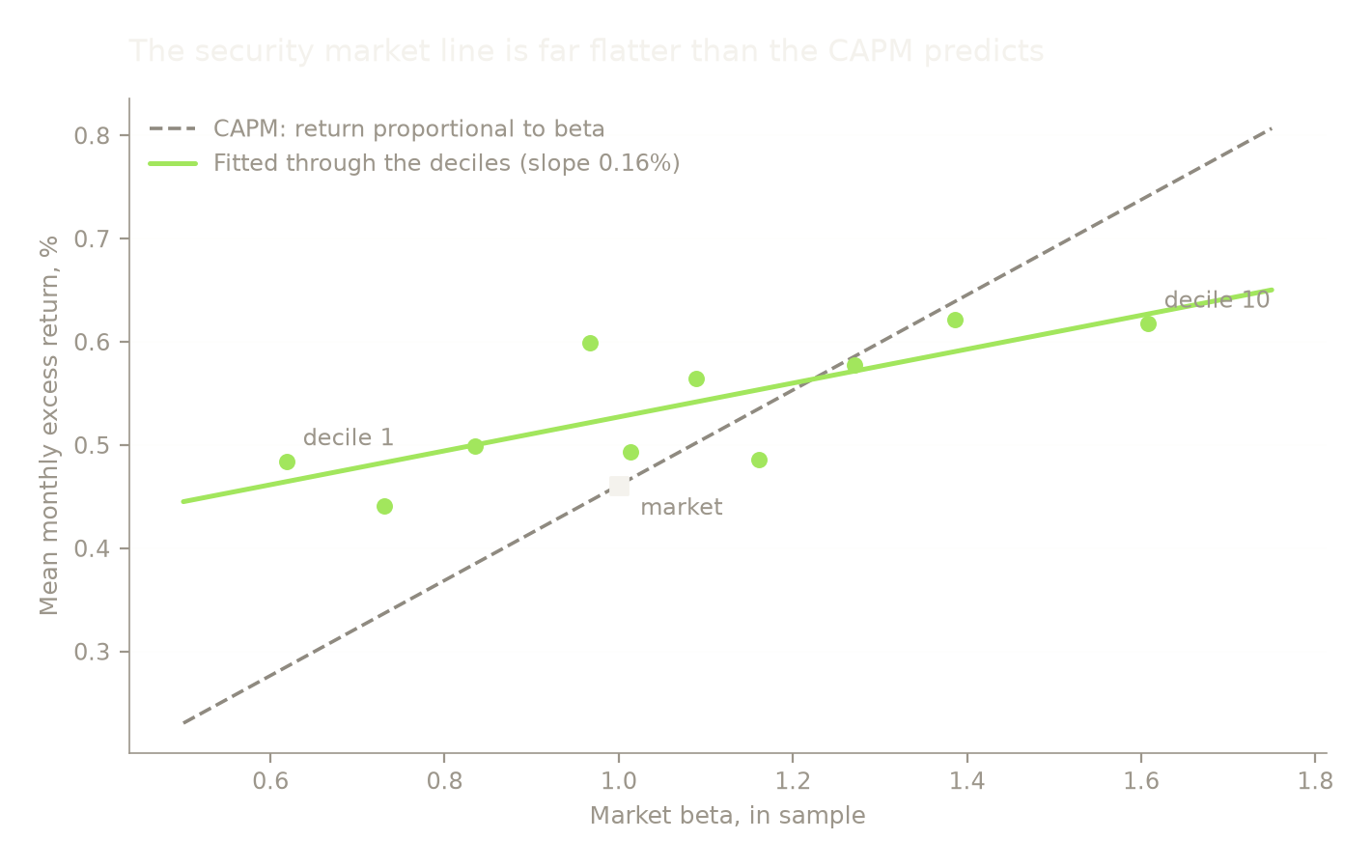
The dashed line is what the CAPM asks for. The solid line is what the deciles actually delivered. The gap between them widens with beta, which is the entire premise of the strategy tested next.
Code16 lines
# Criterion (b): the rescaled long-short, in sample.

bab, w_lo, w_hi, turnover = bab_factor(ex, m["Mkt-RF"])
bab_ins = bab.loc[:"2012-03-31"].dropna()

X = m.loc[bab_ins.index, ["Mkt-RF", "SMB", "HML"]]
fit = capm(bab_ins, X)
sharpe_ins = np.sqrt(12) * bab_ins.mean() / bab_ins.std()

print(f"leverage on the low-beta leg    mean {w_lo.mean():.2f}   max {w_lo.max():.2f}")
print(f"scaling on the high-beta leg    mean {w_hi.mean():.2f}   max {w_hi.max():.2f}")
print(f"monthly weight turnover         mean {turnover.mean():.3f}\n")
print(f"in sample, net of {P['cost_bps']}bp   n {len(bab_ins)} months")
print(f"  mean            {bab_ins.mean():+.3f}% per month")
print(f"  Sharpe          {sharpe_ins:+.3f}")
print(f"  three-factor alpha {fit.params['const']:+.3f}%  t {fit.tvalues['const']:+.2f}")
leverage on the low-beta leg mean 1.70 max 3.26 scaling on the high-beta leg mean 0.63 max 0.78 monthly weight turnover mean 0.035 in sample, net of 10bp n 549 months mean +0.510% per month Sharpe +0.336 three-factor alpha +0.420% t +2.27
Criterion (b) is met, and not by much. The three-factor alpha is +0.42% a month at t = 2.27, against a threshold of 2. The paper reports 0.73% at t = 7.39 on their own factor, so this is roughly half the premium with a fifth of the statistical weight, which is what a coarser sort on a shorter sample should be expected to give.
Leverage averages 1.70 on the low-beta leg and 0.63 on the high-beta leg. That is close to the $1.40 and $0.70 the paper reports for its US factor, so the portfolio being tested here is at least the same shape as theirs.
Code12 lines
fig, ax = plt.subplots(figsize=(8, 4.2))

growth = (1 + bab.dropna() / 100).cumprod()
ax.plot(growth.index, growth.values, color=style.ACCENT, lw=1.6)
ax.axvspan(pd.Timestamp("2012-04-30"), growth.index.max(),
           color=style.SUBTLE, alpha=0.14, lw=0)
ax.annotate("holdout", (pd.Timestamp("2013-06-30"), growth.min() * 1.4),
            fontsize=8.5, color=style.MUTED)
ax.set_yscale("log")
ax.set_ylabel("Growth of $1, log scale")
ax.set_title("Beta-neutral low-minus-high, net of costs")
plt.show()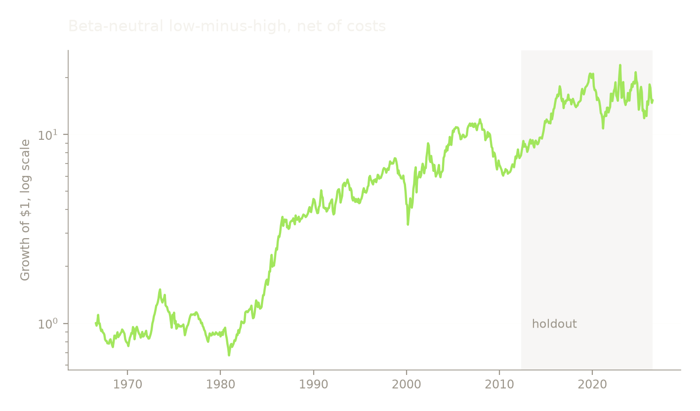
The line is not a smooth climb. Most of the distance is covered in the 1980s and again after 2009, with two long flat stretches in between. The decade panel in What broke puts numbers on that.
Code16 lines
# Criterion (c): the holdout. Evaluated once.

bab_oos = bab.loc["2012-04-30":].dropna()
X_oos = m.loc[bab_oos.index, ["Mkt-RF", "SMB", "HML"]]
fit_oos = capm(bab_oos, X_oos)
sharpe_oos = np.sqrt(12) * bab_oos.mean() / bab_oos.std()

print(f"holdout 2012-04 to 2026-06, net of {P['cost_bps']}bp   n {len(bab_oos)} months")
print(f"  mean            {bab_oos.mean():+.3f}% per month")
print(f"  Sharpe          {sharpe_oos:+.3f}")
print(f"  three-factor alpha {fit_oos.params['const']:+.3f}%  t {fit_oos.tvalues['const']:+.2f}")
print()
print(f"  in sample:  mean {bab_ins.mean():+.3f}%  Sharpe {sharpe_ins:+.3f}  "
      f"alpha {fit.params['const']:+.3f}% (t {fit.tvalues['const']:+.2f})")
print(f"  holdout:    mean {bab_oos.mean():+.3f}%  Sharpe {sharpe_oos:+.3f}  "
      f"alpha {fit_oos.params['const']:+.3f}% (t {fit_oos.tvalues['const']:+.2f})")
holdout 2012-04 to 2026-06, net of 10bp n 171 months mean +0.669% per month Sharpe +0.318 three-factor alpha +0.399% t +0.91 in sample: mean +0.510% Sharpe +0.336 alpha +0.420% (t +2.27) holdout: mean +0.669% Sharpe +0.318 alpha +0.399% (t +0.91)
Criterion (c) is met: the holdout Sharpe ratio is positive, at +0.32 against +0.34 in sample. The mean return is actually higher out of sample than in it, +0.67% a month against +0.51%.
The t-statistic is the part worth being careful about. At 0.91 the holdout alpha is not distinguishable from zero. That is not evidence the premium disappeared, because 171 months at this volatility could not produce a significant t-statistic even if the true alpha were exactly what it was in sample. It does mean the holdout confirms the premium is not obviously gone, and nothing stronger than that.
What broke
Every variant tried, including the ones that fail. All are in sample, net of costs, three-factor alpha with Newey-West standard errors at six lags.
Code31 lines
def variant(label, table=0, cols=None, window=P["post_rank_beta_window_months"],
            cost=P["cost_bps"]):
    cols = cols or DECILES
    d = data.to_month_end(data.famafrench("Portfolios_Formed_on_BETA", AS_OF, table=table))
    mm = d[cols].join(ff[["Mkt-RF", "RF", "SMB", "HML"]], how="inner")
    mm = mm.loc[PREREG["start"]:PREREG["end"]]
    e = mm[cols].sub(mm["RF"], axis=0)
    w_lo = 1.0 / rolling_beta(e[cols[0]],  mm["Mkt-RF"], window=window)
    w_hi = 1.0 / rolling_beta(e[cols[-1]], mm["Mkt-RF"], window=window)
    g = w_lo * e[cols[0]] - w_hi * e[cols[-1]]
    turn = w_lo.diff().abs().fillna(0) + w_hi.diff().abs().fillna(0)
    r = (g - turn * cost / 100.0).loc[:"2012-03-31"].dropna()
    f = capm(r, mm.loc[r.index, ["Mkt-RF", "SMB", "HML"]])
    return (label, len(r), r.mean(), np.sqrt(12) * r.mean() / r.std(),
            f.params["const"], f.tvalues["const"])

QUINTILES = ["Lo 20", "Qnt 2", "Qnt 3", "Qnt 4", "Hi 20"]
variants = [
    variant("preregistered: VW deciles, 60m beta, 10bp"),
    variant("equal-weighted deciles", table=1),
    variant("beta window 36 months", window=36),
    variant("beta window 120 months", window=120),
    variant("quintiles instead of deciles", cols=QUINTILES),
    variant("cost 0bp", cost=0),
    variant("cost 50bp", cost=50),
    variant("cost 100bp", cost=100),
]

print(f"{'variant':44} {'n':>4} {'mean%':>7} {'Sharpe':>7} {'alpha%':>7} {'t':>6}")
for lab, n, mu, sr, a, t in variants:
    print(f"{lab:44} {n:>4} {mu:+7.3f} {sr:+7.3f} {a:+7.3f} {t:+6.2f}")
variant n mean% Sharpe alpha% t preregistered: VW deciles, 60m beta, 10bp 549 +0.510 +0.336 +0.420 +2.27 equal-weighted deciles 549 +0.504 +0.513 +0.382 +2.58 beta window 36 months 549 +0.400 +0.233 +0.273 +1.17 beta window 120 months 549 +0.418 +0.280 +0.264 +1.47 quintiles instead of deciles 549 +0.352 +0.263 +0.261 +1.60 cost 0bp 549 +0.514 +0.339 +0.423 +2.29 cost 50bp 549 +0.495 +0.327 +0.405 +2.19 cost 100bp 549 +0.477 +0.315 +0.386 +2.09
Two of these matter.
The beta window is doing real work. At 36 months the alpha falls to +0.27% with t = 1.17, and at 120 months to +0.26% with t = 1.47. Only the preregistered 60-month window clears the threshold. That window was my choice, not the paper's, which is exactly the kind of parameter that should be suspected when it turns out to be the one that passes. The honest reading is that criterion (b) is met at the specification that was written down in advance, and would not have been met at two nearby specifications.
Deciles are needed. On quintiles the alpha drops to +0.26% with t = 1.60. The premium lives in the tails of the beta distribution, so a coarser sort dilutes it below significance.
Costs are close to irrelevant here, which is a fact about the test rather than about the strategy. Weight turnover averages 0.035 a month, so even 100bp removes only 0.04% a month. The turnover of the underlying deciles is not observable from French's return series and is not charged for at all. A real implementation would pay considerably more than any row in this table.
Code7 lines
# Subperiod behaviour, preregistered specification, net of costs.

print("decade      n    mean%   Sharpe")
for start in range(1960, 2030, 10):
    s = bab.loc[f"{start}":f"{start + 9}"].dropna()
    if len(s) >= 24:
        print(f"{start}s   {len(s):>3}  {s.mean():+7.3f}  {np.sqrt(12) * s.mean() / s.std():+7.2f}")
decade n mean% Sharpe 1960s 42 -0.502 -0.45 1970s 120 +0.166 +0.13 1980s 120 +1.530 +1.06 1990s 120 +0.064 +0.05 2000s 120 +0.652 +0.32 2010s 120 +0.999 +0.82 2020s 78 +0.081 +0.03
Code30 lines
fig, ax = plt.subplots(figsize=(8, 3.9))

labels, means, counts = [], [], []
for start in range(1960, 2030, 10):
    s = bab.loc[f"{start}":f"{start + 9}"].dropna()
    if len(s) >= 24:
        labels.append(f"{start}s")
        means.append(s.mean())
        counts.append(len(s))

# Only the two decades the title is about are loud. Painting every positive
# bar in the accent would make the chart say "mostly positive", which is the
# opposite of the point.
top2 = sorted(range(len(means)), key=lambda i: means[i], reverse=True)[:2]
colors = [style.ACCENT if i in top2 else style.SERIES[2] for i in range(len(means))]

ax.bar(labels, means, color=colors, width=0.62)
ax.axhline(0, color=style.MUTED, lw=0.7)

# Two of these decades are part-period stubs. Without the counts the chart
# would present 42 months and 120 months as equally solid.
for i, (v, n) in enumerate(zip(means, counts)):
    ax.annotate(f"n={n}", (i, 0), textcoords="offset points",
                xytext=(0, -16 if v > 0 else 8), ha="center",
                fontsize=7.5, color=style.MUTED)

ax.set_ylabel("Mean monthly return, %")
ax.set_title("Two decades carry the premium")
ax.tick_params(axis="x", pad=14)
plt.show()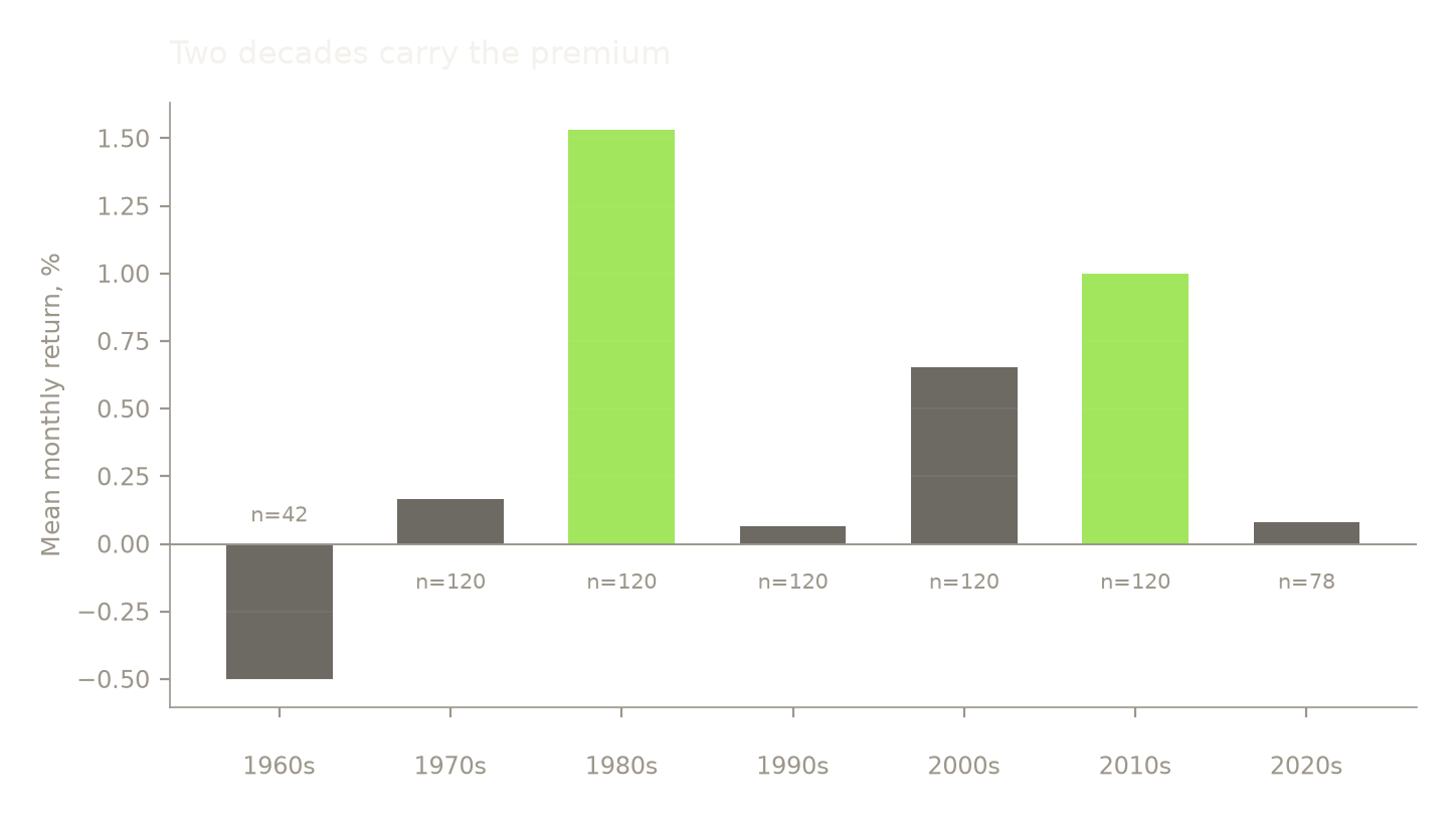
The 1980s deliver +1.53% a month and the 2010s +1.00%. The 1970s and 1990s are close to zero, the 2020s so far are +0.08%, and the 1960s stub is negative on 42 months. A strategy whose record depends this heavily on two decades out of seven is one where a fourteen-year holdout, however it comes out, cannot settle much.
Verdict
The flat security market line replicates decisively and the levered spread replicates weakly. Do not trade this on the strength of this note.
Criterion (a) passes without qualification. Alpha declines almost monotonically across the deciles, the rank correlation is -0.90 at p = 0.0003, and average returns barely rise while beta nearly triples. This part of Frazzini and Pedersen is not in question here.
Criteria (b) and (c) pass as written and are fragile underneath. The in-sample alpha of +0.42% at t = 2.27 clears the threshold, but moving the beta window to 36 or 120 months, or coarsening the sort to quintiles, takes it below. The holdout Sharpe ratio is positive as required, and its t-statistic of 0.91 is too weak to be evidence in either direction. The decade panel shows two decades carrying most of the record.
There is also an explanation this test cannot rule out. Novy-Marx and Velikov argue the BAB premium comes from small illiquid stocks and the factor's weighting scheme rather than from leverage constraints. French's deciles are value-weighted and fixed, so nothing here distinguishes the two stories. A reader who wanted to act on the mechanism would need a test this note does not contain.
What this note does establish is that the flat security market line is still flat, sixty-three years in and fourteen years past the paper that explained it.
References
Black, F., Jensen, M. C. and Scholes, M. (1972). The capital asset pricing model: some empirical tests. In M. C. Jensen (ed.), Studies in the Theory of Capital Markets. New York: Praeger.
Frazzini, A. and Pedersen, L. H. (2014). Betting against beta. Journal of Financial Economics 111(1), 1-25. https://econpapers.repec.org/RePEc:eee:jfinec:v:111:y:2014:i:1:p:1-25 Author copy, which is the text every parameter in this note was read from: https://w4.stern.nyu.edu/facdir/lpederse/papers/BettingAgainstBeta.pdf
French, K. R. (2026). Portfolios formed on BETA; Fama/French 3 factors. Data library, accessed 2026-08-28. https://mba.tuck.dartmouth.edu/pages/faculty/ken.french/data_library.html
McLean, R. D. and Pontiff, J. (2016). Does academic research destroy stock return predictability? Journal of Finance 71(1), 5-32. https://onlinelibrary.wiley.com/doi/10.1111/jofi.12365
Novy-Marx, R. and Velikov, M. (2022). Betting against betting against beta. Journal of Financial Economics 143(1), 80-106. https://pure.psu.edu/en/publications/betting-against-betting-against-beta/
Code6 lines
print(f"python       {sys.version.split()[0]}")
print(f"pandas       {pd.__version__}")
print(f"numpy        {np.__version__}")
print(f"statsmodels  {sm.__version__}")
print(f"seed         {SEED}")
print(f"data as-of   {AS_OF}  (research/data/famafrench/{AS_OF}/)")
python 3.12.13 pandas 3.0.5 numpy 2.5.2 statsmodels 0.15.0 seed 0 data as-of 2026-08-28 (research/data/famafrench/2026-08-28/)