Preregistration — fixed before any data was loaded102 lines
# Frozen before any data was loaded. Every cell below reads from PREREG, so no
# value is typed twice and the plan cannot drift from the code.

PREREG = {
    "hypothesis":
        "The five-factor model of Fama and French (2015) holds up in the 150 "
        "months after that paper's sample ends. Specifically: RMW and CMA "
        "still earn positive premia; HML is still redundant once RMW and CMA "
        "are present; the five-factor model still beats the three-factor "
        "model on the paper's own test portfolios; and the failure the paper "
        "reports on small stocks with low profitability and high investment "
        "is no worse than it was.",

    "universe":
        "Ken French's US 2x3 five-factor series and his 25 Size-B/M, "
        "25 Size-OP, 25 Size-Inv and 32 Size-OP-Inv portfolios. The authors' "
        "own published returns, not a universe rebuilt here.",

    "start": "1963-07-01",
    "end":   "2026-06-30",

    "replication_window":
        "1963-07 to 2013-12, 606 months. The paper's own sample. Used once, "
        "to confirm this pull reproduces its published Tables 4 and 5.",

    "holdout":
        "2014-01 to 2026-06, 150 months. Every month the paper could not "
        "have seen. Touched once, in the last cell of Results.",

    "rebalance":
        "None. French's factors and portfolios are already monthly returns.",

    "params": {
        "as_of": "2026-09-01",
        "factor_file": "F-F_Research_Data_5_Factors_2x3",
        "test_portfolios": {
            "25 Size-B/M":     "25_Portfolios_5x5",
            "25 Size-OP":      "25_Portfolios_ME_OP_5x5",
            "25 Size-Inv":     "25_Portfolios_ME_INV_5x5",
            "32 Size-OP-Inv":  "32_Portfolios_ME_OP_INV_2x4x4",
        },
        "models": {
            "HML":         ["Mkt-RF", "SMB", "HML"],
            "HML RMW":     ["Mkt-RF", "SMB", "HML", "RMW"],
            "HML CMA":     ["Mkt-RF", "SMB", "HML", "CMA"],
            "RMW CMA":     ["Mkt-RF", "SMB", "RMW", "CMA"],
            "HML RMW CMA": ["Mkt-RF", "SMB", "HML", "RMW", "CMA"],
        },
        "t_method":
            "Plain OLS t-statistic on the mean, matching the paper. Table 4's "
            "t-statistics reproduce as mean/(sd/sqrt(n)) to rounding.",
        "nw_lags_robustness": 6,      # author's choice, not the paper's
        "alpha_t_threshold": 2.0,
        "subperiods": {              # robustness only, badly underpowered
            "2014-2019": ("2014-01-01", "2019-12-31"),
            "2020-2026": ("2020-01-01", "2026-06-30"),
        },
    },

    # Table 4, 2x3 factors, 1963-07 to 2013-12, 606 months.
    "paper_table4_2x3": {
        "Mkt-RF": {"mean": 0.50, "sd": 4.49, "t": 2.74},
        "SMB":    {"mean": 0.29, "sd": 3.07, "t": 2.31},
        "HML":    {"mean": 0.37, "sd": 2.88, "t": 3.20},
        "RMW":    {"mean": 0.25, "sd": 2.14, "t": 2.92},
        "CMA":    {"mean": 0.33, "sd": 2.01, "t": 4.07},
    },

    # Table 5, 2x3 factors, 25 Size-B/M portfolios (Panel A). Models are named
    # by the factors beyond Mkt-RF and SMB that they include.
    "paper_table5_2x3_size_bm": {
        "HML":          {"grs": 3.62, "avg_abs_alpha": 0.102},
        "HML RMW":      {"grs": 3.13, "avg_abs_alpha": 0.095},
        "HML CMA":      {"grs": 3.52, "avg_abs_alpha": 0.101},
        "RMW CMA":      {"grs": 2.84, "avg_abs_alpha": 0.100},
        "HML RMW CMA":  {"grs": 2.84, "avg_abs_alpha": 0.094},
    },

    "not_tested":
        "The abstract's claim that performance is insensitive to factor "
        "definition. French publishes only the 2x3 US construction; the 2x2 "
        "and 2x2x2x2 versions in Table 4 are not available, and rebuilding "
        "them would substitute this author's choices for the paper's.",

    "success":
        "Decided per test, before the holdout is opened. "
        "PREMIA: CONTINUED if the holdout 95% confidence interval for a "
        "factor's mean contains the paper's published mean; CHANGED if it "
        "excludes it. "
        "REDUNDANCY: a factor is redundant if the intercept from regressing "
        "it on the other four has |t| below 2.0. "
        "GRS: the five-factor model beats the three-factor model if its GRS "
        "statistic is lower on at least three of the four portfolio sets. "
        "HML is still redundant if dropping it changes GRS by less than the "
        "gap the paper reports between its three- and five-factor models. "
        "SMALL GROWTH: the named failure has worsened if the intercept on "
        "the small, low-profitability, high-investment portfolio is more "
        "negative out of sample than in the replication window. "
        "Significance of any single premium is not the criterion. Minimum "
        "detectable means and implied power are computed from the paper's "
        "own standard deviations and printed before any holdout result.",
}
Setup and imports20 lines
import sys
import warnings

# Library import notices are not findings, and would otherwise be
# published as output. Silenced before the imports that raise them.
warnings.filterwarnings("ignore")


import numpy as np
import pandas as pd
import matplotlib.pyplot as plt
from scipy import stats

sys.path.append("..")
from lib import style
from lib.data import famafrench, to_month_end

style.use()
SEED = 0
np.random.seed(SEED)
Hypothesis
Fama and French published the five-factor model in 2015 on a sample ending in December 2013. This note asks whether the model still describes returns in the 150 months since, none of which the authors could have seen. Four claims from the paper are tested: that the profitability and investment premia are real, that HML becomes redundant once those two are present, that the five-factor model explains the test portfolios better than the three-factor model, and that the model's one admitted failure is confined to small stocks that invest heavily despite low profitability. A premium that has stopped paying, or a redundancy that has reversed, changes how every factor-adjusted result should be read, including the ones published on this site.
Prior work
The paper under test is Fama and French (2015). Its sample, its factor
statistics and its model comparisons are read out of the published article and
recorded in PREREG above, so this note compares against printed numbers
rather than remembered ones.
Two of its sentences fix what is tested here. The first is the redundancy claim: "With the addition of profitability and investment factors, the value factor of the FF three-factor model becomes redundant for describing average returns in the sample we examine." The second is the admission of failure: the model's "main problem is its failure to capture the low average returns on small stocks whose returns behave like those of firms that invest a lot despite low profitability."
A third claim in the same abstract, that "the model's performance is not sensitive to the way its factors are defined", is not tested. French publishes only the 2x3 construction for the United States. The 2x2 and 2x2x2x2 versions exist inside the paper and nowhere in his library, and rebuilding them would replace the authors' construction choices with this author's.
The factor definitions themselves are Fama and French (1993) for the market, size and value factors, extended in the 2015 paper with operating profitability and investment. The test statistic for the model comparisons is Gibbons, Ross and Shanken (1989).
Data
Everything comes from Ken French's data library, pulled once and cached under
research/data/famafrench/2026-09-01/. Every cell reads the cache, never the
network, so the numbers below survive French's monthly rebuild of his files.
Five monthly series and four sets of test portfolios. The factors are the 2x3 construction, which is the one the paper leads with and the only one French publishes for the United States. Returns are in percent per month. Portfolio returns are converted to excess returns by subtracting the one-month Treasury bill rate carried in the same factor file.
There is no survivorship bias to declare. These are the authors' own published factor and portfolio returns, not a universe reconstructed here from today's index membership. The point-in-time question does not arise for the same reason: French builds each month's portfolios from information available at that month's formation date.
One caveat belongs here rather than further down. The paper was written against French's 2014 vintage of these files, and he has rebuilt them every month since. The replication cell in Method measures how far today's vintage has moved from the numbers the paper printed.
Code19 lines
AS_OF = PREREG["params"]["as_of"]

factors = to_month_end(famafrench(PREREG["params"]["factor_file"], AS_OF, 0))
portfolios = {
    label: to_month_end(famafrench(name, AS_OF, 0))
    for label, name in PREREG["params"]["test_portfolios"].items()
}

REP = slice(PREREG["start"], "2013-12-31")     # the paper's own months
OOS = slice("2014-01-01", PREREG["end"])       # months it could not have seen

print(f"factors      {factors.index.min():%Y-%m} to {factors.index.max():%Y-%m}"
      f"  n={len(factors)}  cols={list(factors.columns)}")
for label, df in portfolios.items():
    print(f"{label:16} {df.index.min():%Y-%m} to {df.index.max():%Y-%m}"
          f"  n={len(df)}  portfolios={df.shape[1]}")
print()
print(f"replication  n={len(factors.loc[REP])} months")
print(f"holdout      n={len(factors.loc[OOS])} months")
factors 1963-07 to 2026-06 n=756 cols=['Mkt-RF', 'SMB', 'HML', 'RMW', 'CMA', 'RF'] 25 Size-B/M 1926-07 to 2026-06 n=1200 portfolios=25 25 Size-OP 1963-07 to 2026-06 n=756 portfolios=25 25 Size-Inv 1963-07 to 2026-06 n=756 portfolios=25 32 Size-OP-Inv 1963-07 to 2026-06 n=756 portfolios=32 replication n=606 months holdout n=150 months
Method
Four tests, each with a published number to be measured against.
Premia. The mean, standard deviation and t-statistic of each factor. The
paper's t-statistics reproduce as mean / (sd / sqrt(n)), so they are plain
rather than autocorrelation-corrected, and the same form is used here. A
Newey-West version appears in What broke.
Redundancy. Each factor regressed on the other four. The intercept is the part of that factor's average return the others cannot explain. An intercept indistinguishable from zero means the factor adds nothing to the model.
Model comparison. The GRS statistic of Gibbons, Ross and Shanken tests whether the intercepts across a whole set of test portfolios are jointly zero. Lower is better: a model with nothing left over has no intercepts to find.
The admitted failure. The paper names one portfolio type it cannot price. The intercept on that corner is compared between windows.
The power calculation comes first and is not optional. A 150-month window is short for measuring a factor premium, and the arithmetic below decides in advance which questions this sample can answer at all.
Code47 lines
def t_stat(x):
    """Plain t-statistic on a mean, matching the paper's Table 4."""
    x = np.asarray(x, dtype=float)
    return x.mean() / (x.std(ddof=1) / np.sqrt(len(x)))


def newey_west_t(x, lags):
    """Autocorrelation-robust t on a mean. Robustness only, not the primary test."""
    x = np.asarray(x, dtype=float)
    n = len(x)
    e = x - x.mean()
    gamma0 = (e @ e) / n
    var = gamma0
    for k in range(1, lags + 1):
        gk = (e[k:] @ e[:-k]) / n
        var += 2 * (1 - k / (lags + 1)) * gk
    return x.mean() / np.sqrt(var / n)


def grs(excess, F):
    """Gibbons, Ross & Shanken (1989).

    `excess` is T x N test-asset excess returns, `F` is T x K factor returns.
    Returns the statistic, its p-value, and the average absolute intercept.
    """
    R = np.asarray(excess, dtype=float)
    Fv = np.asarray(F, dtype=float)
    T, N = R.shape
    K = Fv.shape[1]
    X = np.column_stack([np.ones(T), Fv])
    B = np.linalg.lstsq(X, R, rcond=None)[0]
    alpha = B[0]
    resid = R - X @ B
    Sigma = (resid.T @ resid) / (T - K - 1)
    mu = Fv.mean(axis=0)
    Omega = np.cov(Fv, rowvar=False, ddof=1)
    sharpe_sq = mu @ np.linalg.solve(np.atleast_2d(Omega), mu)
    stat = ((T - N - K) / N) * (alpha @ np.linalg.solve(Sigma, alpha)) / (1 + sharpe_sq)
    p = stats.f.sf(stat, N, T - N - K)
    return stat, p, np.abs(alpha).mean()


def detectable(sd, n, threshold):
    """Smallest mean this many months could call significant, and the power
    to detect a premium that simply continued at the paper's published size."""
    se = sd / np.sqrt(n)
return se * threshold, seCode22 lines
# What 150 months can and cannot answer, computed from the paper's own
# standard deviations before any holdout number is read.
n_oos = len(factors.loc[OOS])
thr = PREREG["params"]["alpha_t_threshold"]

rows = []
for name, pub in PREREG["paper_table4_2x3"].items():
    mde, se = detectable(pub["sd"], n_oos, thr)
    t_if_unchanged = pub["mean"] / se
    power = stats.norm.sf(thr - t_if_unchanged)
    rows.append({
        "factor": name,
        "paper mean": pub["mean"],
        "paper sd": pub["sd"],
        "min detectable mean": round(mde, 3),
        "t if unchanged": round(t_if_unchanged, 2),
        "power at |t|>2": round(power, 2),
    })

power_table = pd.DataFrame(rows).set_index("factor")
print(f"holdout n = {n_oos} months\n")
print(power_table.to_string())
holdout n = 150 months
paper mean paper sd min detectable mean t if unchanged power at |t|>2
factor
Mkt-RF 0.50 4.49 0.733 1.36 0.26
SMB 0.29 3.07 0.501 1.16 0.20
HML 0.37 2.88 0.470 1.57 0.33
RMW 0.25 2.14 0.349 1.43 0.28
CMA 0.33 2.01 0.328 2.01 0.50
Code14 lines
# Does today's vintage of French's files still produce the paper's Table 4?
rep = factors.loc[REP]
rows = []
for name, pub in PREREG["paper_table4_2x3"].items():
    x = rep[name]
    rows.append({
        "factor": name,
        "mean": round(x.mean(), 2),      "paper mean": pub["mean"],
        "sd": round(x.std(ddof=1), 2),   "paper sd": pub["sd"],
        "t": round(t_stat(x), 2),        "paper t": pub["t"],
    })
replication = pd.DataFrame(rows).set_index("factor")
print(f"1963-07 to 2013-12, n = {len(rep)} (paper: 606)\n")
print(replication.to_string())
1963-07 to 2013-12, n = 606 (paper: 606)
mean paper mean sd paper sd t paper t
factor
Mkt-RF 0.50 0.50 4.48 4.49 2.75 2.74
SMB 0.28 0.29 3.05 3.07 2.25 2.31
HML 0.38 0.37 2.79 2.88 3.37 3.20
RMW 0.26 0.25 2.25 2.14 2.89 2.92
CMA 0.33 0.33 2.00 2.01 4.01 4.07
Code17 lines
# The same check for Table 5: model comparisons on the 25 Size-B/M portfolios.
rep_f = factors.loc[REP]
rep_p = portfolios["25 Size-B/M"].loc[REP]
rep_ex = rep_p.sub(rep_f["RF"], axis=0)

rows = []
for label, cols in PREREG["params"]["models"].items():
    g, p, aa = grs(rep_ex, rep_f[cols])
    pub = PREREG["paper_table5_2x3_size_bm"][label]
    rows.append({
        "model": label,
        "GRS": round(g, 2),        "paper GRS": pub["grs"],
        "A|a|": round(aa, 3),      "paper A|a|": pub["avg_abs_alpha"],
    })
replication_grs = pd.DataFrame(rows).set_index("model")
print(f"25 Size-B/M, 1963-07 to 2013-12, n = {len(rep_ex)}\n")
print(replication_grs.to_string())
25 Size-B/M, 1963-07 to 2013-12, n = 606
GRS paper GRS A|a| paper A|a|
model
HML 3.55 3.62 0.098 0.102
HML RMW 3.18 3.13 0.093 0.095
HML CMA 3.47 3.52 0.097 0.101
RMW CMA 3.04 2.84 0.094 0.100
HML RMW CMA 3.06 2.84 0.093 0.094
Results
Code22 lines
# The holdout is opened here and read once.
oos_f = factors.loc[OOS]

rows = []
for name, pub in PREREG["paper_table4_2x3"].items():
    x = oos_f[name]
    m, sd, n = x.mean(), x.std(ddof=1), len(x)
    se = sd / np.sqrt(n)
    lo, hi = m - 1.96 * se, m + 1.96 * se
    contains = lo <= pub["mean"] <= hi
    rows.append({
        "factor": name,
        "paper mean": pub["mean"],
        "holdout mean": round(m, 2),
        "95% low": round(lo, 2),
        "95% high": round(hi, 2),
        "t": round(t_stat(x), 2),
        "verdict": "CONTINUED" if contains else "CHANGED",
    })
premia = pd.DataFrame(rows).set_index("factor")
print(f"2014-01 to 2026-06, n = {len(oos_f)} months\n")
print(premia.to_string())
2014-01 to 2026-06, n = 150 months
paper mean holdout mean 95% low 95% high t verdict
factor
Mkt-RF 0.50 1.00 0.30 1.70 2.81 CONTINUED
SMB 0.29 -0.19 -0.65 0.28 -0.78 CHANGED
HML 0.37 -0.04 -0.62 0.53 -0.14 CONTINUED
RMW 0.25 0.14 -0.23 0.50 0.74 CONTINUED
CMA 0.33 -0.08 -0.45 0.29 -0.41 CHANGED
Code26 lines
FACTORS = list(PREREG["paper_table4_2x3"])

def redundancy(window_f, label):
    rows = []
    for target in FACTORS:
        others = [c for c in FACTORS if c != target]
        y = window_f[target].values
        X = np.column_stack([np.ones(len(y)), window_f[others].values])
        beta, *_ = np.linalg.lstsq(X, y, rcond=None)
        resid = y - X @ beta
        dof = len(y) - X.shape[1]
        s2 = (resid @ resid) / dof
        se = np.sqrt(s2 * np.linalg.inv(X.T @ X)[0, 0])
        t = beta[0] / se
        rows.append({
            "factor": target,
            "intercept": round(beta[0], 3),
            "t": round(t, 2),
            "redundant": abs(t) < PREREG["params"]["alpha_t_threshold"],
        })
    return pd.DataFrame(rows).set_index("factor").add_suffix(f" [{label}]")

red_rep = redundancy(factors.loc[REP], "1963-2013")
red_oos = redundancy(oos_f, "2014-2026")
print("Each factor regressed on the other four.\n")
print(red_rep.join(red_oos).to_string())
Each factor regressed on the other four.
intercept [1963-2013] t [1963-2013] redundant [1963-2013] intercept [2014-2026] t [2014-2026] redundant [2014-2026]
factor
Mkt-RF 0.813 4.92 False 1.024 3.07 False
SMB 0.360 3.02 False -0.292 -1.43 True
HML -0.009 -0.10 True 0.057 0.26 True
RMW 0.431 5.03 False 0.039 0.22 True
CMA 0.255 4.54 False 0.018 0.12 True
Code19 lines
def grs_table(window):
    out = {}
    for pf_label, df in portfolios.items():
        f_w = factors.loc[window]
        ex = df.loc[window].sub(f_w["RF"], axis=0)
        ex = ex.replace(-99.99, np.nan).dropna(axis=1, how="any")
        col = {}
        for m_label, cols in PREREG["params"]["models"].items():
            g, p, aa = grs(ex, f_w[cols])
            col[m_label] = round(g, 2)
        out[f"{pf_label} (N={ex.shape[1]})"] = col
    return pd.DataFrame(out)

grs_rep = grs_table(REP)
grs_oos = grs_table(OOS)
print("GRS statistic, lower is better. Replication window:\n")
print(grs_rep.to_string())
print("\nHoldout:\n")
print(grs_oos.to_string())
GRS statistic, lower is better. Replication window:
25 Size-B/M (N=25) 25 Size-OP (N=25) 25 Size-Inv (N=25) 32 Size-OP-Inv (N=32)
HML 3.55 2.27 4.54 4.12
HML RMW 3.18 1.61 4.38 3.60
HML CMA 3.47 2.87 4.01 3.67
RMW CMA 3.04 1.87 3.50 2.89
HML RMW CMA 3.06 1.87 3.49 2.89
Holdout:
25 Size-B/M (N=25) 25 Size-OP (N=25) 25 Size-Inv (N=25) 32 Size-OP-Inv (N=32)
HML 1.20 1.17 0.91 1.03
HML RMW 1.22 1.27 0.92 1.07
HML CMA 1.18 1.19 0.90 1.02
RMW CMA 1.23 1.32 0.89 1.03
HML RMW CMA 1.21 1.30 0.91 1.05
Code28 lines
# The failure the paper names: small stocks, low profitability, high investment.
# In the 2x4x4 sort that is the small size group, lowest OP quartile, highest
# Inv quartile. French labels these "SMALL LoOP HiINV" or a close variant.
sm = portfolios["32 Size-OP-Inv"]
corner = [c for c in sm.columns if c.strip().upper().startswith("SMALL")
          and "LOOP" in c.replace(" ", "").upper()
          and "HIINV" in c.replace(" ", "").upper()]
print("candidate columns:", corner if corner else list(sm.columns[:8]))

five = PREREG["params"]["models"]["HML RMW CMA"]

def corner_alpha(window, col):
    f_w = factors.loc[window]
    y = (sm.loc[window, col] - f_w["RF"]).values
    X = np.column_stack([np.ones(len(y)), f_w[five].values])
    beta, *_ = np.linalg.lstsq(X, y, rcond=None)
    resid = y - X @ beta
    dof = len(y) - X.shape[1]
    se = np.sqrt((resid @ resid) / dof * np.linalg.inv(X.T @ X)[0, 0])
    return beta[0], beta[0] / se

col = corner[0]
a_rep, t_rep = corner_alpha(REP, col)
a_oos, t_oos = corner_alpha(OOS, col)
print(f"\nportfolio: {col!r}")
print(f"five-factor intercept, 1963-2013 : {a_rep:+.3f} %/month  (t = {t_rep:+.2f})")
print(f"five-factor intercept, 2014-2026 : {a_oos:+.3f} %/month  (t = {t_oos:+.2f})")
print(f"worsened: {a_oos < a_rep}")
candidate columns: ['SMALL LoOP HiINV'] portfolio: 'SMALL LoOP HiINV' five-factor intercept, 1963-2013 : -0.482 %/month (t = -6.07) five-factor intercept, 2014-2026 : +0.093 %/month (t = +0.50) worsened: False
Code29 lines
# The holdout only. Plotting from 1963 compresses the 150 months this note is
# about into a sliver, and the question is not what the factors did over sixty
# years, it is whether they kept paying after the paper went out. Dotted lines
# are what the paper's published means would have compounded to over the same
# months, so the gap between solid and dotted is the finding.
fig, ax = plt.subplots(figsize=(8.0, 4.2))

oos_cum = (1 + factors.loc[OOS, ["RMW", "CMA", "HML"]] / 100).cumprod()
months = np.arange(1, len(oos_cum) + 1)

# Colours are set per factor rather than through `style.emphasise`, which walks
# every line on the axes and would recolour each dotted reference away from the
# solid line it belongs to. A reader has to be able to pair them by eye.
PAIRS = [("RMW", style.ACCENT, 1.8), ("CMA", style.SERIES[1], 1.0),
         ("HML", style.SERIES[2], 1.0)]

for name, colour, width in PAIRS:
    ax.plot(oos_cum.index, oos_cum[name], color=colour, lw=width,
            zorder=3 if colour == style.ACCENT else 2, label=name)
    implied = (1 + PREREG["paper_table4_2x3"][name]["mean"] / 100) ** months
    ax.plot(oos_cum.index, implied, color=colour, lw=0.9, ls=(0, (2, 2)),
            alpha=0.55, zorder=1)

ax.axhline(1.0, color=style.MUTED, lw=0.6, alpha=0.5)
ax.set_ylabel("growth of 1, from January 2014")
ax.set_title("What the three factors paid after the paper was published")
ax.legend(loc="upper left", title="solid: actual   dotted: paper's mean")
style.check_points(ax)
plt.show()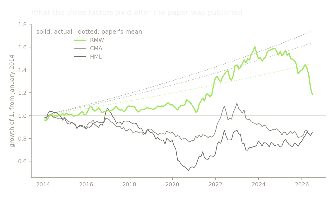
Code29 lines
# One portfolio set, the paper's own Panel A, so the bars line up with a
# published number. The dashed line is where GRS stops being distinguishable
# from zero intercepts at 5%; a bar below it means nothing is left to explain.
fig, ax = plt.subplots(figsize=(8.0, 4.2))

col_rep = grs_rep["25 Size-B/M (N=25)"]
col_oos = grs_oos["25 Size-B/M (N=25)"]
labels = list(col_oos.index)
x = np.arange(len(labels))
w = 0.38

ax.bar(x - w / 2, col_rep.values, w, color=style.SERIES[2], label="1963-2013")
ax.bar(x + w / 2, col_oos.values, w, color=style.ACCENT, label="2014-2026")

crit = stats.f.ppf(0.95, 25, len(factors.loc[OOS]) - 25 - 5)
ax.axhline(crit, color=style.MUTED, lw=0.9, ls=(0, (4, 3)))
ax.annotate(f"5% critical value ({crit:.2f})", xy=(-0.45, crit),
            xytext=(0, 5), textcoords="offset points", ha="left",
            fontsize=8, color=style.MUTED)

ax.set_xticks(x)
ax.set_xticklabels(labels, rotation=20, ha="right")
ax.set_ylabel("GRS, 25 Size-B/M portfolios")
ax.set_title("Does the model leave less unexplained than it used to?")
# Headroom first, then a two-column legend above the bars. At the default
# limits the legend box sat on top of the tallest bar.
ax.set_ylim(0, 4.4)
ax.legend(loc="upper center", ncol=2)
plt.show()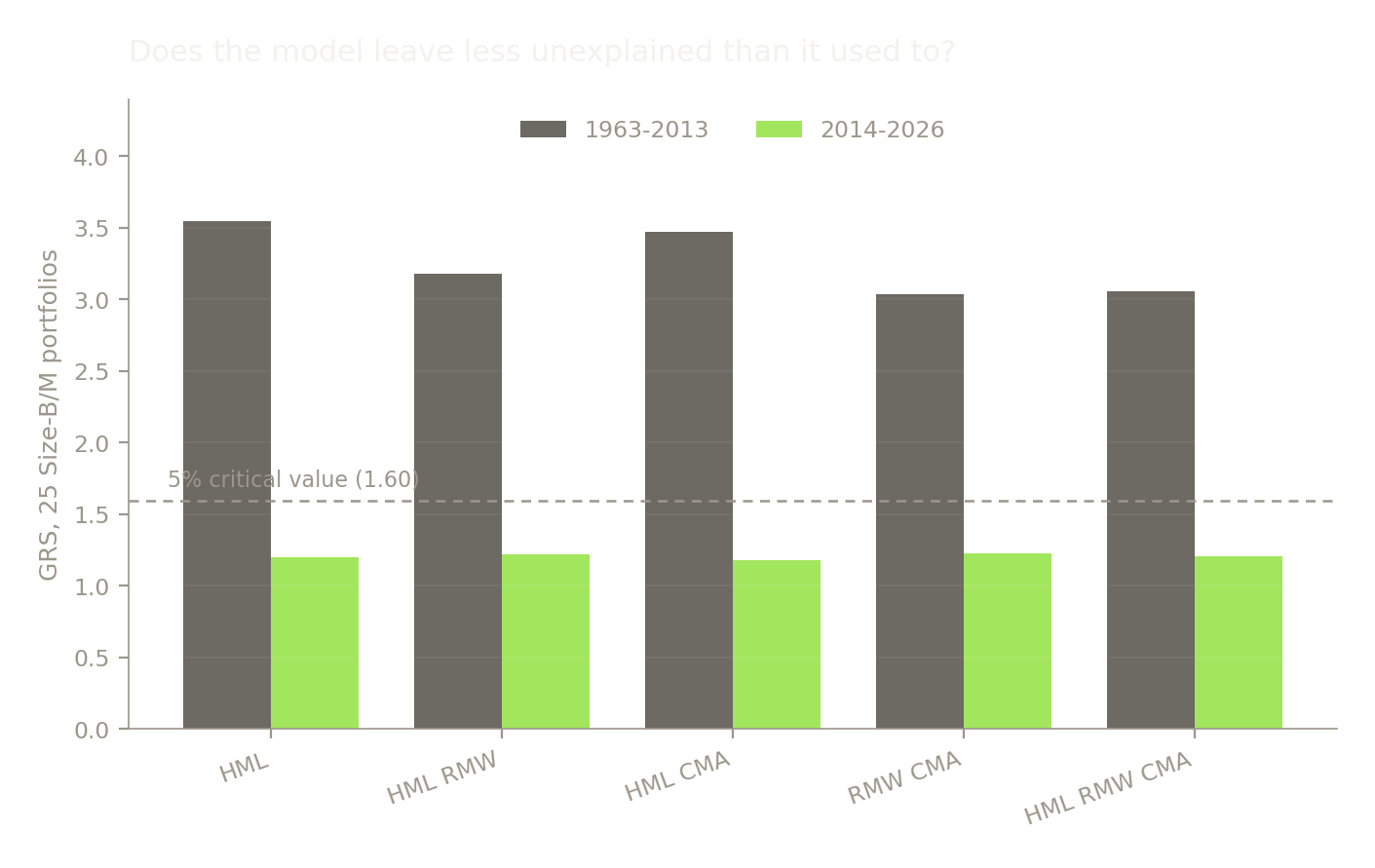
What broke
Everything tried after the preregistration was frozen, including the versions that did not survive.
Code11 lines
rows = []
lags = PREREG["params"]["nw_lags_robustness"]
for name in FACTORS:
    x = oos_f[name]
    rows.append({
        "factor": name,
        "plain t": round(t_stat(x), 2),
        f"Newey-West t ({lags} lags)": round(newey_west_t(x, lags), 2),
    })
print("Autocorrelation correction. Not the primary test; the paper does not use one.\n")
print(pd.DataFrame(rows).set_index("factor").to_string())
Autocorrelation correction. Not the primary test; the paper does not use one.
plain t Newey-West t (6 lags)
factor
Mkt-RF 2.81 3.71
SMB -0.78 -0.80
HML -0.14 -0.12
RMW 0.74 0.73
CMA -0.41 -0.40
Code14 lines
# Splitting 150 months in half leaves each piece badly underpowered. This is
# here because it was preregistered, not because either half decides anything.
rows = []
for label, (a, b) in PREREG["params"]["subperiods"].items():
    w = factors.loc[a:b]
    for name in FACTORS:
        rows.append({
            "period": label, "n": len(w), "factor": name,
            "mean": round(w[name].mean(), 2),
            "t": round(t_stat(w[name]), 2),
        })
sub = pd.DataFrame(rows).pivot(index="factor", columns="period",
                               values=["mean", "t"])
print(sub.to_string())
mean t period 2014-2019 2020-2026 2014-2019 2020-2026 factor CMA -0.20 0.04 -1.14 0.12 HML -0.31 0.20 -1.04 0.41 Mkt-RF 0.91 1.09 2.25 1.89 RMW 0.14 0.14 0.79 0.44 SMB -0.25 -0.13 -0.84 -0.35
Code23 lines
# End-point sensitivity. The holdout stops in the middle of a sharp RMW
# drawdown: April, May and June 2026 ran -4.30, -8.42 and -4.64. A mean
# measured to the last available month inherits that, so here is the same mean
# with the tail trimmed. This was not preregistered; it is here because the
# data showed it.
rows = []
for cut in [0, 3, 6, 12]:
    w = oos_f.iloc[: len(oos_f) - cut] if cut else oos_f
    row = {"months dropped": cut, "n": len(w)}
    for name in FACTORS:
        row[name] = round(w[name].mean(), 2)
    rows.append(row)
print("Holdout mean with the final months removed.\n")
print(pd.DataFrame(rows).set_index("months dropped").to_string())


# Vintage drift: how far today's files have moved from the paper's 2014 pull.
drift = replication.copy()
drift["mean gap"] = (drift["mean"] - drift["paper mean"]).round(2)
drift["sd gap"] = (drift["sd"] - drift["paper sd"]).round(2)
drift["sd gap %"] = (100 * drift["sd gap"] / drift["paper sd"]).round(1)
print("Same months, same construction, twelve years of rebuilds apart.\n")
print(drift[["mean gap", "sd gap", "sd gap %"]].to_string())
Holdout mean with the final months removed.
n Mkt-RF SMB HML RMW CMA
months dropped
0 150 1.00 -0.19 -0.04 0.14 -0.08
3 147 0.93 -0.21 -0.04 0.26 -0.07
6 144 0.99 -0.24 -0.11 0.25 -0.12
12 138 0.97 -0.27 -0.16 0.31 -0.08
Same months, same construction, twelve years of rebuilds apart.
mean gap sd gap sd gap %
factor
Mkt-RF 0.00 -0.01 -0.2
SMB -0.01 -0.02 -0.7
HML 0.01 -0.09 -3.1
RMW 0.01 0.11 5.1
CMA 0.00 -0.01 -0.5
Verdict
The model is not broken. On these portfolios and in these months it is unnecessary, which is a different finding and a more awkward one.
The premia are undecided, and were always going to be. By the preregistered rule, SMB and CMA CHANGED: their holdout confidence intervals exclude the means the paper published. Mkt-RF, HML and RMW CONTINUED. That word is doing less work than it looks. HML averaged -0.04% a month against a published 0.37%, and still counts as continued only because 150 months put a confidence interval around it more than a percentage point wide. The power table printed before the holdout was opened says why: no factor here reaches even a coin flip's chance of registering its own published premium as significant, and the market factor, the strongest of them, gets 26%. A note that read these five rows as five deaths would be reporting the sample size, not the world.
RMW deserves a second sentence. Its holdout mean of 0.14% is measured to a sample that stops in the middle of a three-month fall of -4.30, -8.42 and -4.64. Ending the window three months earlier puts it at 0.26%, against the 0.25% the paper published. The profitability premium did not fade across these twelve years so much as give a large part of itself back in the final quarter of them, and which of those two sentences is true is not something 150 months can settle. That check appears in What broke and was not preregistered; the data suggested it.
Redundancy spread. In the paper's own window only HML was redundant, which is what the paper says. In the holdout, HML, SMB, RMW and CMA are all redundant: regress any one of them on the other four and the intercept cannot be told from zero. Only the market factor survives that test. The paper's sentence about the value factor becoming redundant now describes four of its five factors.
No model beat any other. The five-factor model does not clear the preregistered bar of a lower GRS on at least three of the four portfolio sets. It does not beat the three-factor model on any of them. The reason is not that it failed but that nothing failed: every GRS in the holdout sits between 0.89 and 1.32, below the 5% critical value, so the intercepts are jointly indistinguishable from zero under all five specifications including the simplest. There is no mispricing left in these portfolios for an extra factor to pick up.
The failure the paper admitted to has gone. Small stocks with low profitability and high investment carried a five-factor intercept of -0.48% a month with a t of -6.07 across 1963 to 2013, which is the anomaly the abstract names as the model's main problem. Across 2014 to 2026 that intercept is +0.09% with a t of 0.50. Whatever was wrong there is no longer measurable.
What to do with it. For factor-adjusting US portfolio returns since 2014, the choice between three and five factors changes almost nothing, and the choice between either and the market alone changes less than the literature implies. Anyone quoting a five-factor alpha on a post-2014 US sample is quoting a number that a one-factor regression would have produced too. That is worth knowing before it is used as evidence.
None of this says the profitability and investment premia are gone. It says this sample cannot see them, that the portfolios they were built to price no longer need them, and that twelve and a half years is not long enough to settle the first question. The next test worth running is the same one outside the United States, where the sample is independent rather than merely longer.
References
Fama, E. F., & French, K. R. (2015). A five-factor asset pricing model. Journal of Financial Economics, 116(1), 1-22. https://www.sciencedirect.com/science/article/abs/pii/S0304405X14002323
Fama, E. F., & French, K. R. (1993). Common risk factors in the returns on stocks and bonds. Journal of Financial Economics, 33(1), 3-56. https://ideas.repec.org/a/eee/jfinec/v33y1993i1p3-56.html
Gibbons, M. R., Ross, S. A., & Shanken, J. (1989). A test of the efficiency of a given portfolio. Econometrica, 57(5), 1121-1152. https://ideas.repec.org/a/ecm/emetrp/v57y1989i5p1121-52.html
Publisher pages for these two are behind checks that refuse an automated fetch, so the RePEc records are cited instead. Each was fetched and its title matched before publishing. The 2015 paper's own text was read from a copy hosted at INSEAD, which is where its sample period and Tables 4 and 5 were taken from.
French, K. R. (2026). Fama/French 5 factors (2x3); 25 portfolios formed on size and book-to-market; 25 portfolios formed on size and operating profitability; 25 portfolios formed on size and investment; 32 portfolios formed on size, operating profitability and investment. Data library, accessed 2026-09-01. https://mba.tuck.dartmouth.edu/pages/faculty/ken.french/data_library.html
Code8 lines
import matplotlib, scipy
print(f"python      {sys.version.split()[0]}")
print(f"pandas      {pd.__version__}")
print(f"numpy       {np.__version__}")
print(f"scipy       {scipy.__version__}")
print(f"matplotlib  {matplotlib.__version__}")
print(f"seed        {SEED}")
print(f"data as-of  famafrench {AS_OF}")
python 3.10.9 pandas 2.3.1 numpy 1.23.5 scipy 1.10.0 matplotlib 3.7.0 seed 0 data as-of famafrench 2026-09-01