Preregistration — fixed before any data was loaded67 lines
# Frozen before any data is loaded. Every cell below reads from PREREG,
# so no value is typed twice and the plan cannot drift from the code.
#
# Provenance of every parameter.
#
# From Sloan (1996), The Accounting Review 71(3), 289-315, read out of the
# JSTOR scan:
#   - the sort variable: accruals, scaled by average total assets
#   - ten portfolios, low accrual minus high accrual as the hedge portfolio
#   - his sample is Compustat NYSE and AMEX firm-years, 1962 through 1991
#   - returns are measured starting four months after fiscal year end
#
# From Green, Hand & Soliman (2011), Management Science 57(5), 797-816,
# abstract read on the INFORMS page:
#   - the claim under test: the hedge returns to Sloan's accruals anomaly
#     have decayed "to the point that they are, on average, no longer
#     reliably positive"
#
# Mine, not theirs, and named as mine:
#   - the three period boundaries. Both are publication dates, which are
#     facts, rather than either paper's sample end, which would put the
#     boundary at a date the market could not have known.
#   - cost_bps, hac_lags, and the decision rule in "success".
#
# French's AC/B is not Sloan's accrual measure. His is the change in
# operating working capital per split-adjusted share from t-2 to t-1 over
# book equity per share at t-1; Sloan's is balance-sheet accruals over
# average total assets. Decay is therefore measured within this one series
# across time and never against Sloan's printed hedge return.

PREREG = {
    "hypothesis": (
        "The low-minus-high accrual decile spread on Ken French's "
        "accrual-sorted portfolios earned a positive average monthly return "
        "before Sloan was published, and its average in the period after "
        "Green, Hand and Soliman declared the anomaly gone is lower and no "
        "longer reliably different from zero."
    ),
    "universe": (
        "Ken French Portfolios_Formed_on_AC, value-weighted deciles built "
        "from NYSE, AMEX and NASDAQ common stocks on CRSP, formed each June "
        "on AC/B. Equal-weighted deciles are the preregistered robustness "
        "cut, because Sloan's result was equal-weighted. Built from CRSP, so "
        "no survivorship bias enters through universe selection."
    ),
    "start":     "1963-07-31",
    "end":       "2026-06-30",
    "holdout":   "2011-05-31 onwards, touched once in the last cell of Results",
    "rebalance": "annual, French forms the portfolios at the end of June",
    "params": {
        "n_deciles":        10,
        "pre_pub_end":      "1996-06-30",   # month before Sloan, TAR 71(3), July 1996
        "interim_end":      "2011-04-30",   # month before Green/Hand/Soliman, MS 57(5), May 2011
        "cost_bps":         20,
        "hac_lags":         12,
        "min_months":       60,
    },
    "success": (
        "Both must hold for the decay claim to replicate. (a) Over "
        "1963-07 to 1996-06 the value-weighted low-minus-high spread has a "
        "positive mean monthly return with |t| > 2 under Newey-West standard "
        "errors, net of 20bp round-trip costs. (b) In the holdout the net "
        "mean is below the pre-publication mean and its |t| is under 2. "
        "If (a) fails, the note reports that the anomaly was never present "
        "in this series and the decay question does not arise."
    ),
}
Setup and imports22 lines
import sys
import warnings

# Library import notices are not findings, and they would otherwise be
# published as output. Silenced before the imports that raise them.
warnings.filterwarnings("ignore")

import numpy as np
import pandas as pd
import statsmodels.api as sm
import matplotlib.pyplot as plt

sys.path.append("..")
from lib import style, data

style.use()
SEED = 0
np.random.seed(SEED)

AS_OF = "2026-08-28"          # as-of date of every cached pull in this note
P = PREREG["params"]
DECILES = ["Lo 10"] + [f"Dec {i}" for i in range(2, 10)] + ["Hi 10"]
Hypothesis
Firms whose earnings lean on accruals rather than cash go on to disappoint, and a portfolio long low-accrual stocks and short high-accrual stocks used to be paid for knowing that. It is not paid any more.
Sloan (1996) documented the pattern. Green, Hand and Soliman (2011) reported that it had stopped working, and attributed that to hedge fund capital moving into the trade. This note tests both claims on Ken French's accrual-sorted deciles: that the spread was reliably positive before Sloan was published, and that in the fifteen years since Green, Hand and Soliman it is no longer distinguishable from zero.
The test was fixed before any data was loaded. It is in the first cell, including the period boundaries, which are publication dates rather than either paper's sample end, and the success criterion.
Prior work
Sloan, R. G. (1996). Do stock prices fully reflect information in accruals and cash flows about future earnings? The Accounting Review 71(3), 289-315. The original. He sorts on accruals scaled by average total assets, forms ten portfolios, and measures returns from four months after fiscal year end so the financial statements are public. His sample is Compustat NYSE and AMEX firm-years from 1962 through 1991.
Green, J., Hand, J. R. M. and Soliman, M. T. (2011). Going, going, gone? The apparent demise of the accruals anomaly. Management Science 57(5), 797-816. The claim under test. They report the hedge returns "appear to have decayed in U.S. stock markets to the point that they are, on average, no longer reliably positive", and attribute it partly to hedge fund capital entering the trade.
McLean, R. D. and Pontiff, J. (2016). Does academic research destroy stock return predictability? Journal of Finance 71(1), 5-32. The general version of the same claim across 97 predictors, with an average post-publication decline of 58%. It is the reason the period boundaries here are publication dates: if publication is the mechanism, the boundary belongs where the information became public, not where a sample happened to end.
Data
Ken French's data library, cached on 2026-08-28 under
research/data/famafrench/. Two series: the monthly accrual-sorted portfolios
and the monthly research factors. All returns are in percent.
French builds the portfolios from CRSP himself, so no survivorship bias enters through universe selection.
Three things a reader should hold against this test.
French's accrual measure is not Sloan's. French sorts on AC/B: the change in operating working capital per split-adjusted share from t-2 to t-1, divided by book equity per share at t-1. Sloan uses balance-sheet accruals, defined as the change in non-cash current assets less the change in current liabilities excluding short-term debt and taxes payable, minus depreciation, all scaled by average total assets. These are related but not the same variable. Every comparison below is therefore made within this one series across time. Sloan's printed hedge return is never used as a benchmark, because a gap against it would measure the difference in construction rather than any change in the world.
The default here is value-weighted, Sloan's result was equal-weighted. Value-weighted is French's default and is the harder test, since an equal-weighted spread leans on small stocks. The equal-weighted version is preregistered and appears in What broke.
Costs are a rough floor. French forms these portfolios once a year at the end of June, so the round trip is charged once a year, in July. Holdings are not published, so within-year drift and the actual cost of trading the tails are not captured.
Code11 lines
dec = data.to_month_end(data.famafrench("Portfolios_Formed_on_AC", AS_OF, table=0))
ff  = data.to_month_end(data.famafrench("F-F_Research_Data_Factors", AS_OF))

m = dec[DECILES].join(ff[["Mkt-RF", "RF", "SMB", "HML"]], how="inner")
m = m.loc[PREREG["start"]:PREREG["end"]]
ex = m[DECILES].sub(m["RF"], axis=0)          # excess returns, percent per month

print(f"deciles  {len(dec):6,} rows  {dec.index.min().date()} -> {dec.index.max().date()}")
print(f"factors  {len(ff):6,} rows  {ff.index.min().date()} -> {ff.index.max().date()}")
print(f"merged   {len(m):6,} rows  {m.index.min().date()} -> {m.index.max().date()}")
print(f"missing values in the merged panel: {int(m.isna().sum().sum())}")
deciles 756 rows 1963-07-31 -> 2026-06-30 factors 1,200 rows 1926-07-31 -> 2026-06-30 merged 756 rows 1963-07-31 -> 2026-06-30 missing values in the merged panel: 0
Method
The strategy is long the lowest-accrual decile and short the highest, held for a year, rebuilt each June when French rebuilds the portfolios. The round trip is charged once a year, in July, at the preregistered 20bp.
Three periods, split at publication dates:
- before Sloan, 1963-07 to 1996-06
- between the two papers, 1996-07 to 2011-04
- the holdout, 2011-05 onward, touched once
Means are tested against zero with Newey-West standard errors at twelve lags. Twelve rather than six because the portfolios are annually rebalanced, so overlapping information persists for about a year.
The decay claim needs both halves. If the spread was never positive in this series, then there is nothing to have decayed, and the note reports that instead.
Code22 lines
def hedge(table=0, cols=None, cost_bps=P["cost_bps"]):
    """Low-accrual minus high-accrual, with the annual round trip charged in
    July, the month after French rebuilds the portfolios."""
    cols = cols or DECILES
    d = data.to_month_end(data.famafrench("Portfolios_Formed_on_AC", AS_OF, table=table))
    mm = d[cols].join(ff[["Mkt-RF", "RF", "SMB", "HML"]], how="inner")
    mm = mm.loc[PREREG["start"]:PREREG["end"]]
    gross = mm[cols[0]] - mm[cols[-1]]
    charge = pd.Series(0.0, index=mm.index)
    charge[mm.index.month == 7] = 2 * cost_bps / 100.0   # out of one leg, into the other
    return gross - charge, mm

def mean_t(r, lags=P["hac_lags"]):
    """Mean and its Newey-West t-statistic against zero."""
    fit = sm.OLS(r.values, np.ones(len(r))).fit(cov_type="HAC", cov_kwds={"maxlags": lags})
    return len(r), r.mean(), float(fit.tvalues[0]), np.sqrt(12) * r.mean() / r.std()

spread, m = hedge()
PERIODS = [
    ("before Sloan        1963-07 to 1996-06", slice(None, P["pre_pub_end"])),
    ("between the papers  1996-07 to 2011-04", slice("1996-07-01", P["interim_end"])),
]
Results
Code9 lines
# Criterion (a): was the spread there before Sloan was published?

print("low-accrual minus high-accrual decile, value-weighted, net of costs\n")
print(f"{'period':40} {'n':>4} {'mean%':>8} {'t':>7} {'Sharpe':>8}")
for label, sl in PERIODS:
    n, mu, t, sr = mean_t(spread.loc[sl])
    print(f"{label:40} {n:>4} {mu:+8.3f} {t:+7.2f} {sr:+8.3f}")
n, mu, t, sr = mean_t(spread)
print(f"{'full sample         1963-07 to 2026-06':40} {n:>4} {mu:+8.3f} {t:+7.2f} {sr:+8.3f}")
low-accrual minus high-accrual decile, value-weighted, net of costs period n mean% t Sharpe before Sloan 1963-07 to 1996-06 396 +0.379 +3.14 +0.504 between the papers 1996-07 to 2011-04 178 +0.187 +0.88 +0.197 full sample 1963-07 to 2026-06 756 +0.261 +2.50 +0.310
Criterion (a) is met. Before Sloan was published the spread paid +0.38% a month at t = 3.14, net of costs, with an annualised Sharpe ratio of 0.50.
Between the two papers the mean falls to +0.19% at t = 0.88. That average hides a turn rather than describing a steady decline: the strategy was still paying well for the first eight of those years and flat for the rest. The growth chart below shows where the change actually happened.
Code20 lines
fig, ax = plt.subplots(figsize=(8, 4.4))

pre  = ex.loc[:P["pre_pub_end"]].mean()
hold = ex.loc["2011-05-01":].mean()
x = np.arange(1, 11)

# Demeaned within each period. Raw means are not comparable across periods:
# the holdout is a bull market, which lifts all ten deciles together and would
# hide the only thing being compared, which is the slope.
ax.plot(x, pre - pre.mean(), color=style.ACCENT, lw=1.8, marker="o", ms=4,
        label="Before Sloan, 1963-07 to 1996-06")
ax.plot(x, hold - hold.mean(), color=style.SERIES[1], lw=1.2, marker="o", ms=4,
        label="Holdout, 2011-05 to 2026-06")
ax.axhline(0, color=style.MUTED, lw=0.7)
ax.set_xticks(x)
ax.set_xlabel("Accrual decile, 1 = lowest accruals")
ax.set_ylabel("Mean monthly excess return\nrelative to the period average, %")
ax.set_title("The accrual sort used to slope down. It no longer does.")
ax.legend(loc="lower left")
plt.show()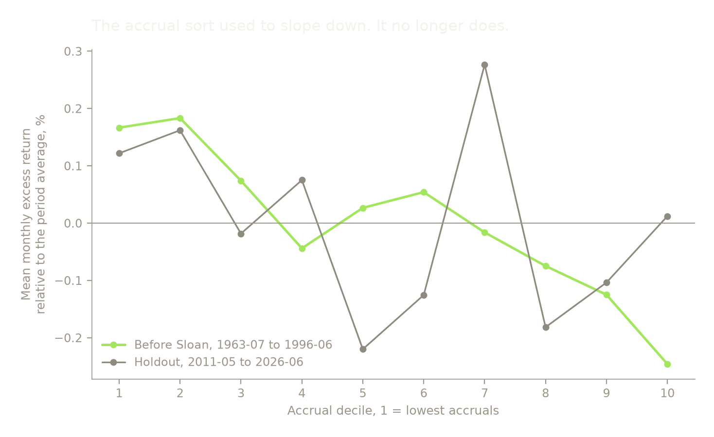
The accent line falls from left to right, which is the anomaly: low-accrual deciles beat high-accrual deciles by about 0.4% a month across the sort. The grey line is close to flat and its highest point is decile 7, which is where a sort carrying no information would put it.
Code16 lines
fig, ax = plt.subplots(figsize=(8, 4.2))

growth = (1 + spread / 100).cumprod()
ax.plot(growth.index, growth.values, color=style.ACCENT, lw=1.6)

# Linear, not log. The series spans about 6x, and a log axis over that range
# only buys a set of minor tick labels nobody reads.
for date, label, height in [("1996-07-31", "Sloan", 0.94),
                            ("2011-05-31", "Green, Hand and Soliman", 0.10)]:
    ax.axvline(pd.Timestamp(date), color=style.SERIES[1], lw=1.0, ls="--")
    ax.annotate(label, (pd.Timestamp(date), growth.max() * height),
                textcoords="offset points", xytext=(6, 0),
                fontsize=8.5, color=style.MUTED)
ax.set_ylabel("Growth of $1")
ax.set_title("Long low-accrual, short high-accrual, net of costs")
plt.show()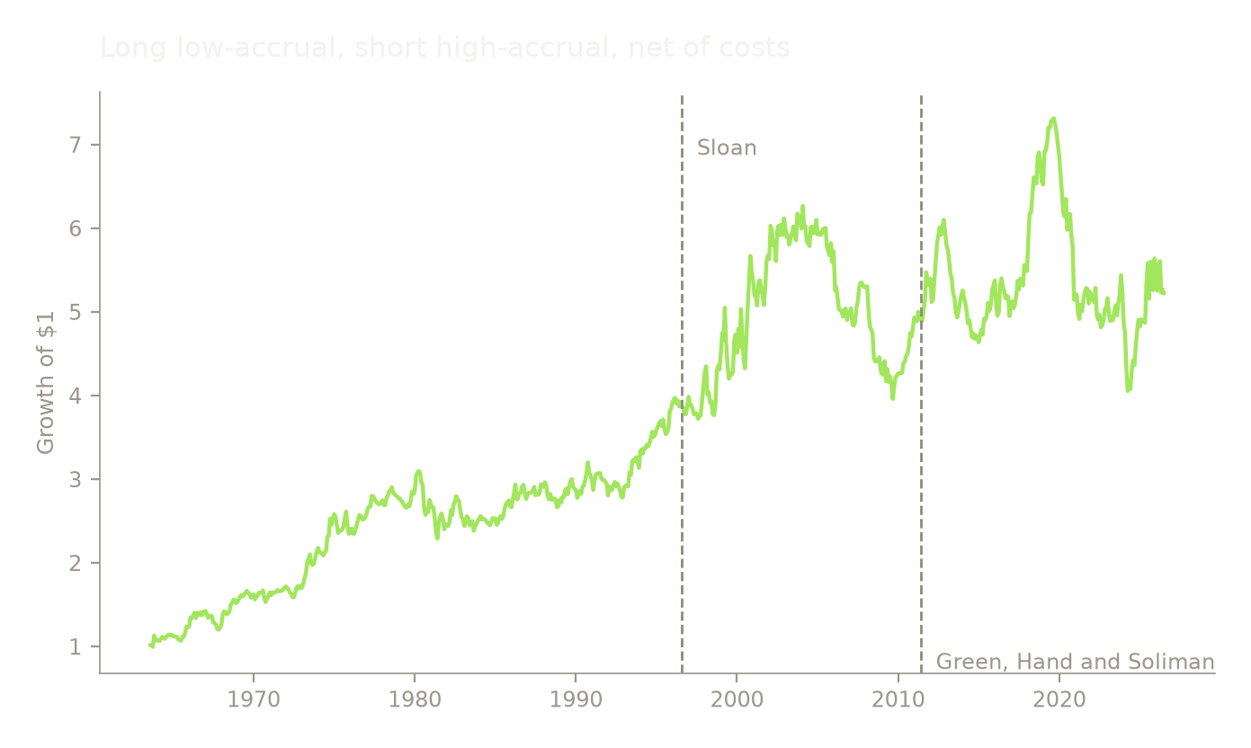
A dollar grows to 3.92 by the month Sloan was published and carries on to 6.27 by January 2004. Over the twenty-two years since, it has ranged between 3.96 and 7.31 and ends at 5.22, below where it stood in 2004.
Neither dashed line marks the turn. The strategy paid well for about eight years after Sloan appeared, and it had already stopped seven years before Green, Hand and Soliman published. Whatever ended it, the timing does not line up with either paper.
Code14 lines
# Criterion (b): the holdout. Evaluated once.

hold_r = spread.loc["2011-05-01":]
n_h, mu_h, t_h, sr_h = mean_t(hold_r)
n_p, mu_p, t_p, sr_p = mean_t(spread.loc[:P["pre_pub_end"]])

print(f"holdout 2011-05 to 2026-06, net of {P['cost_bps']}bp   n {n_h} months")
print(f"  mean    {mu_h:+.3f}% per month")
print(f"  t       {t_h:+.2f}")
print(f"  Sharpe  {sr_h:+.3f}")
print()
print(f"  before Sloan:  mean {mu_p:+.3f}%  t {t_p:+.2f}  Sharpe {sr_p:+.3f}")
print(f"  holdout:       mean {mu_h:+.3f}%  t {t_h:+.2f}  Sharpe {sr_h:+.3f}")
print(f"  the spread retains {100 * mu_h / mu_p:.0f}% of its pre-publication mean")
holdout 2011-05 to 2026-06, net of 20bp n 182 months mean +0.077% per month t +0.29 Sharpe +0.084 before Sloan: mean +0.379% t +3.14 Sharpe +0.504 holdout: mean +0.077% t +0.29 Sharpe +0.084 the spread retains 20% of its pre-publication mean
Criterion (b) is met. The holdout mean is +0.08% a month at t = 0.29, against +0.38% at t = 3.14 before publication. About a fifth of the original premium remains and it is indistinguishable from zero.
Both halves of the preregistered claim therefore hold on this series. The anomaly was real, and it is gone.
What broke
Every variant tried, reported against both the pre-publication period and the holdout.
Code17 lines
QUINTILES = ["Lo 20", "Qnt 2", "Qnt 3", "Qnt 4", "Hi 20"]
variants = [
    ("preregistered: VW deciles, 20bp", dict()),
    ("equal-weighted deciles",          dict(table=1)),
    ("quintiles instead of deciles",    dict(cols=QUINTILES)),
    ("cost 0bp",                        dict(cost_bps=0)),
    ("cost 100bp",                      dict(cost_bps=100)),
]

print(f"{'variant':34} {'pre n':>6} {'pre%':>7} {'pre t':>6}   "
      f"{'hold n':>6} {'hold%':>7} {'hold t':>7}")
for label, kw in variants:
    r, _ = hedge(**kw)
    a = mean_t(r.loc[:P["pre_pub_end"]])
    b = mean_t(r.loc["2011-05-01":])
    print(f"{label:34} {a[0]:>6} {a[1]:+7.3f} {a[2]:+6.2f}   "
          f"{b[0]:>6} {b[1]:+7.3f} {b[2]:+7.2f}")
variant pre n pre% pre t hold n hold% hold t preregistered: VW deciles, 20bp 396 +0.379 +3.14 182 +0.077 +0.29 equal-weighted deciles 396 +0.387 +4.23 182 +0.194 +0.90 quintiles instead of deciles 396 +0.349 +3.49 182 +0.133 +0.72 cost 0bp 396 +0.413 +3.42 182 +0.110 +0.41
cost 100bp 396 +0.246 +2.04 182 -0.055 -0.21
The conclusion does not move. Equal-weighting raises the pre-publication t-statistic to 4.23, which is expected since Sloan's own result was equal-weighted and the effect is stronger in small stocks, and its holdout t-statistic is still 0.90. Quintiles weaken it as a coarser sort should. Costs are close to irrelevant on an annually rebalanced portfolio: at 100bp the pre-publication spread still clears t = 2.
Code8 lines
# Subperiod behaviour, preregistered specification.

print("decade      n    mean%       t")
for start in range(1960, 2030, 10):
    s = spread.loc[f"{start}":f"{start + 9}"]
    if len(s) >= 24:
        _, mu, t, _ = mean_t(s)
        print(f"{start}s   {len(s):>3}  {mu:+7.3f}  {t:+6.2f}")
decade n mean% t 1960s 78 +0.668 +2.09 1970s 120 +0.500 +2.43 1980s 120 +0.040 +0.20 1990s 120 +0.420 +2.56 2000s 120 +0.005 +0.02 2010s 120 +0.426 +1.57 2020s 78 -0.276 -0.65
Code25 lines
fig, ax = plt.subplots(figsize=(8, 3.9))

labels, means, counts = [], [], []
for start in range(1960, 2030, 10):
    s = spread.loc[f"{start}":f"{start + 9}"]
    if len(s) >= 24:
        labels.append(f"{start}s")
        means.append(s.mean())
        counts.append(len(s))

# The decades that clear t = 2 on their own are the loud ones. Everything
# else is context, including the positive-but-insignificant bars.
sig = [abs(mean_t(spread.loc[f"{lab[:4]}":f"{int(lab[:4]) + 9}"])[2]) > 2 for lab in labels]
colors = [style.ACCENT if s else style.SERIES[2] for s in sig]

ax.bar(labels, means, color=colors, width=0.62)
ax.axhline(0, color=style.MUTED, lw=0.7)
for i, (v, n) in enumerate(zip(means, counts)):
    ax.annotate(f"n={n}", (i, 0), textcoords="offset points",
                xytext=(0, -16 if v > 0 else 8), ha="center",
                fontsize=7.5, color=style.MUTED)
ax.set_ylabel("Mean monthly return, %")
ax.set_title("Decades reaching t > 2 on their own, in accent")
ax.tick_params(axis="x", pad=14)
plt.show()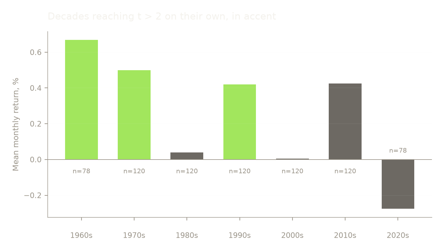
This is the result that complicates the paper's explanation. If hedge fund capital arbitraged the anomaly away after Sloan published in 1996, the decade pattern should be a decline. It is not. The 1980s returned +0.04% a month and the 2000s +0.01%, both long before and after publication respectively, while the 1990s returned +0.42% and the 2010s +0.43%. The premium was already absent for a decade in the middle of the pre-publication period.
The three-period split and the decade panel are both true, and they support different stories. The split says the anomaly decayed. The decade panel says it was intermittent throughout and the last fifteen years look like the 1980s looked. Nothing in this note separates a premium that was arbitraged away from one that was never stable.
Verdict
Do not trade it. Both preregistered criteria are met, so Green, Hand and Soliman's claim replicates on French's accrual-sorted deciles.
The spread paid +0.38% a month at t = 3.14 before Sloan was published, and +0.08% at t = 0.29 in the fifteen years after Green, Hand and Soliman declared it finished. About a fifth of the premium is left and it is not distinguishable from zero. The decile sort, which used to slope down cleanly from low accruals to high, is now flat with its peak in decile 7.
What the note does not establish is why. The decade panel shows two near-zero decades inside the period when the anomaly was supposedly working, which is hard to square with publication or with hedge fund capital as the cause. A reader looking for the mechanism will not find it here. A reader asking whether to allocate to it will: on this series there has been nothing to allocate to since the mid-1990s.
References
French, K. R. (2026). Portfolios formed on AC; Fama/French 3 factors. Data library, accessed 2026-08-28. https://mba.tuck.dartmouth.edu/pages/faculty/ken.french/data_library.html
Green, J., Hand, J. R. M. and Soliman, M. T. (2011). Going, going, gone? The apparent demise of the accruals anomaly. Management Science 57(5), 797-816. https://pubsonline.informs.org/doi/abs/10.1287/mnsc.1110.1320
McLean, R. D. and Pontiff, J. (2016). Does academic research destroy stock return predictability? Journal of Finance 71(1), 5-32. https://onlinelibrary.wiley.com/doi/10.1111/jofi.12365
Sloan, R. G. (1996). Do stock prices fully reflect information in accruals and cash flows about future earnings? The Accounting Review 71(3), 289-315. The publisher's page is not reachable without a subscription. The copy read for this note, and the one every parameter above was taken from, is the scan at https://www.cuhk.edu.hk/acy2/workshop/June2009Wasley/1996TAR).pdf
Code6 lines
print(f"python       {sys.version.split()[0]}")
print(f"pandas       {pd.__version__}")
print(f"numpy        {np.__version__}")
print(f"statsmodels  {sm.__version__}")
print(f"seed         {SEED}")
print(f"data as-of   {AS_OF}  (research/data/famafrench/{AS_OF}/)")
python 3.12.13 pandas 3.0.5 numpy 2.5.2 statsmodels 0.15.0 seed 0 data as-of 2026-08-28 (research/data/famafrench/2026-08-28/)